10 Week 10: Reporting, Reproducibility and Workflow
Objective of this session:
Learn how to produce (interactive) reports, export and format layouts
Learn how to collaborate more efficiently with others
Learn how to make your analysis reproducible
Learn how to set up a workflow that saves you time
This week I will take some more time to first talk about some important concepts in the social sciences and data sciences more generally: reporting and reproducibility. Then I will bring this back together and teach you how R handles these issues through Rmarkdown. At the end, we need to talk about workflow. Rmarkdown introduces a new type of file or script, so the question is: how does it relate to R scripts which we have been dealing with up to now?
R commands covered in this session:
- Rmarkdown
10.1 Reporting
Up to this week, we have been busy managing and wrangling our data, understanding it by using descriptive statistics, producing tables and plots. We covered a lot and you can pad yourself on the back (no one can see you anyways).
In the exercises that you were asked to do each week, I usually presented you with a scenario: Somebody from the university administration approaches you (the data analyst) and asks you questions about students at the university (the data that we have been using). We dug into the data and pulled out the information we needed. We produced single statistics like counts, averages etc. as well as tables and figures.
But something we have not covered is how we actually get that information to whoever is asking. How do we report our findings? What we would have done up to now is probably just copy and paste or even screenshot some statistics or plots into an email or into a word document, added some text and explanations and then send it off. In practice, this is actually done a lot. But it is not recommended. It is clunky, messy, error-prone and a lot of manual work especially if your reports get longer. If something changes in your report, you must run your new code and copy paste the results manually again into a new document or email. Imagine you just get the x-axis label wrong and then you have to do it over again.
Tip: Different outlets (journals, websites, books, course instructors) have different standards on what needs to be reported for different analyses. For example, some journals like you to report the minimum and maximum value for every continuous variable in your summary table, other may not. Make sure you check what is expected of you before producing your outputs.
Copy pasting things from R manually and pasting them somewhere has not only a higher risk of human error and additional work, but it is also less reproducible.
10.2 Reproducibility
Reproducibility is the degree to which your work is easily reproducible by someone else. Why does this matter? Well, imagine you get promoted into a more senior data analyst position because everyone has been impressed with your work. You are joining a team of people at the president’s office that already work on data projects. You are asked to update a previous report with new student data. This can be a nightmare when the previous report left you messy, unreproducible code. You waste a lot of time trying to understand what has been done before. If only they provided you with reproducible and well-annotated code. Let’s all make a plea right now to always keep our code tidy and reproducible for the wellbeing of all analysts in the world.
There is also another reason. Imagine the previous person messed up and there are issues with the code. The previous report was actually wrong. If the code was reproducible, you can easily go through it and understand what happened and possibly correct the mistake. With most data analysis projects, it is always good to have more eyes on the code than just yours.
Many sciences (social and natural) have recently suffered from “reproducibility” or “replication” crisis. Scientists try to work towards truth. Yet, when researchers tried to repeat studies that were published in renowned journals, they were not able to do so. Even when running the code provided by the authors in their respective studies, replication often failed. The results that were reported in the study could not be reproduced by the same code script. This can happen accidentally or on purpose. In either case, it is a big problem. Just as an unfalsifiable theory is a bad theory, non-reproducible results are suspicious results at best and untrustworthy at worst. As a result, there is now growing pressure on researchers to make their research transparent and 100% reproducible.
Reproducibility is not only an issue in the sciences. Imagine you work for a tech start-up or for a newspaper. Projects in the private sectors are often more collaborative and many staff departments work together to develop single elements of a larger analysis. Each element has to be reproducible by all people involved. Before a report is released or a graphic put in a newspaper, others will – or at least should – double-check the code behind the analysis to make sure it is correct.
Garret Grolemund – one of the authors of Rmarkdown – says it much better than I can. Watch the first 10 min of this video. It is worth it. Rmarkdown was developed to present a “turning point” in the discussion on the “replication crisis.”
Ok – we got an idea of why it is there, but what is it?
10.3 What is Markdown?
Rmarkdown is a (fairly easy) R tool to produce rich, fully documented, reproducible, interactive reports for various formats (html, word, pdf) by combining text, code and outputs (tables, plots) all in one file. While it has certain drawbacks (more on that later), Rmarkdown is very flexible and can be used to format, layout and produce very different looking reports. It does not stop there, you can use Rmarkdown applications to produce blogs, journal papers, websites, interactive applications. Let’s take a look here.
Spoiler: This whole course has been implemented using Rmarkdown!
Rmarkdown lets you combine various parts of R (code, output windows etc.) with prose (text). It brings together the console and the script editor, blurring the lines between interactive exploration and long-term code capture.
As I mentioned above, Rmarkdown uses a new type of file or script, with a different structure and way of writing code. So, the question becomes how does it relate to R scripts which we have been dealing with up to now?
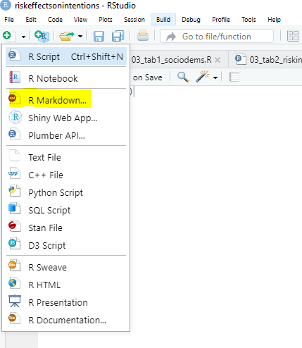
You open an Rmarkdown file through File -> New File -> Rmarkdown or by clicking on the page plus symbol on the upper left-hand corner of R Studio. Try it! Go to R Studio and open one:
R will ask you for a name of the project, your name and a type of file you want to produce. For the file type, let’s select html for now.
What is html? Wikipedia tells us that HTML or Hyper Text Markup Language (HTML) is a markup language for creating a webpage. Markup languages are different from programming languages such as R, insofar they do not serve the purpose of manipulating or generating new data. Markup languages are solely used to define in predetermined ways how to represent data. Webpages are usually viewed in a web browser. They can include writing, links, pictures, and even sound and video. HTML is used to specify how each of these kinds of content are to be displayed in the web browser. We will use html to produce a report, not a website (for now). The advantage of html is that you can display more things compared to word, particularly interactive things. More on that later.
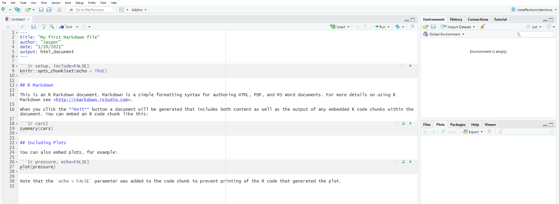
When you have the Rmarkdown file open, you will notice it looks quite different, right? The white-and-grey stripes appear because as mentioned above, R Markdown allows for text and R code to be used in the same document. This means, simply put, that all the white chunks are where you write your text as you would in Microsoft Word (we will talk about formatting later on). Meanwhile, in the grey chunks, you can write code (they are handily called code chunks) and include any output like graphs and tables at the exact point in the text where you would like them to be in the end. Don’t worry, the final output document has no resemblance of a zebra and you can even hide and show your code chunks as you wish!
You are probably wondering how Rmarkdown files relate to R scripts that we have used to write code for our analysis in the previous weeks. Now, there are very different ways to organizing your work and how you link scripts and markdown files (see section on workflow below). There is no right or wrong way. It depends on the project and, to some degree, on the preferences of the person.
My preference more generally, but also for this course, is to keep separate. Think of R scripts as the place where you produce outputs. Then think of Rmarkdown as the tool to “export” and “communicate” your outputs.
10.4 Application in R
10.4.1 Main elements of Rmarkdown
There are generally three large elements in Rmarkdown:
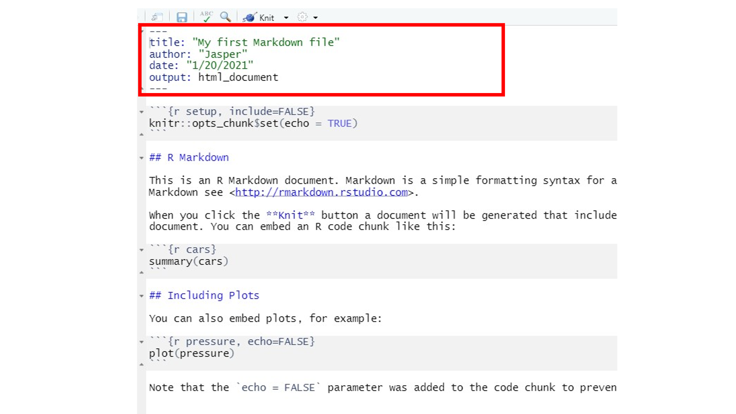
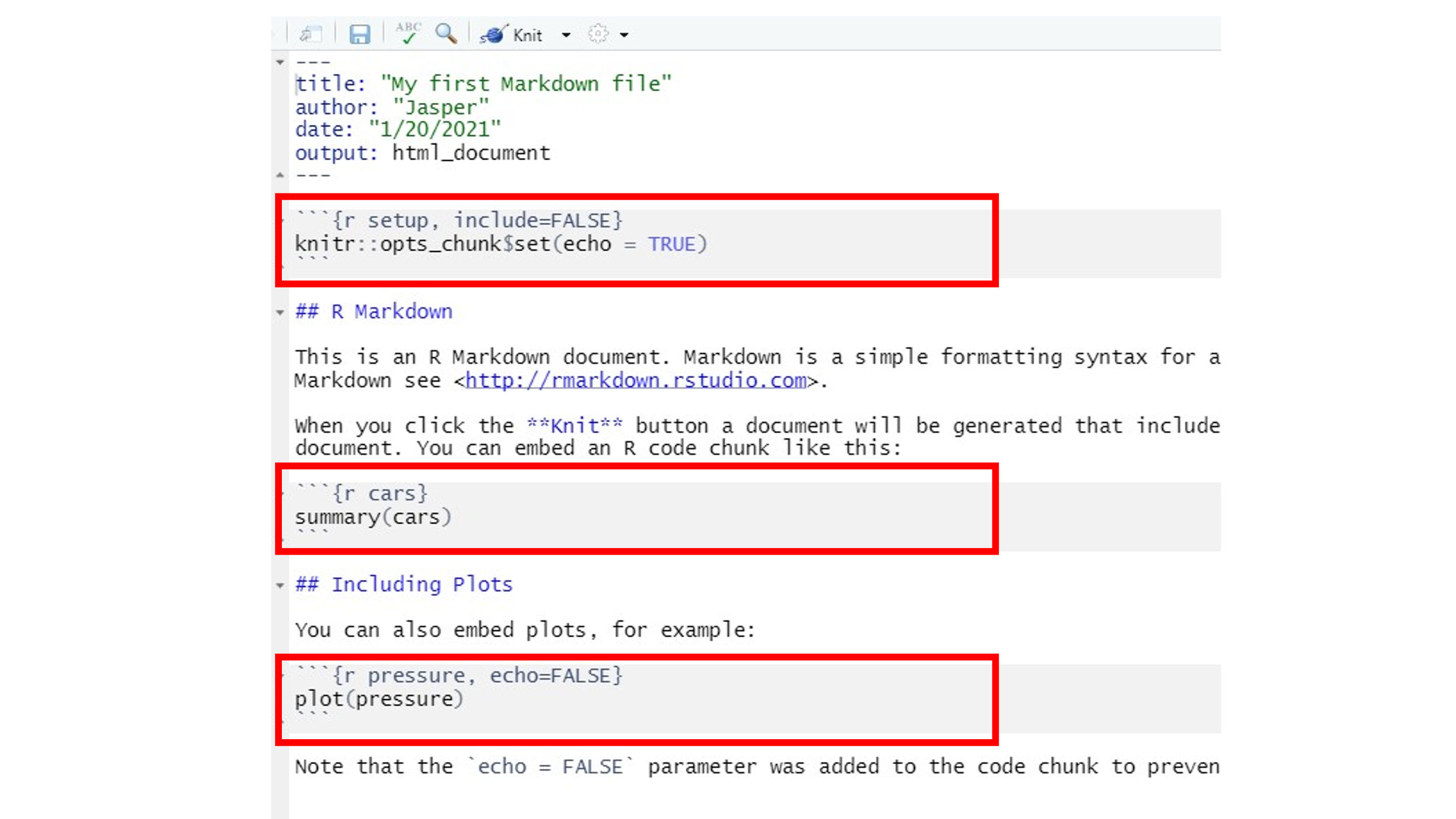
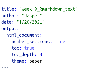
- YAML header: YAML is a human-readableB data-serialization language. Right. It doesn’t really matter what it is, but what it does. The YAML header is at the top of every Rmarkdown document. Here you define basic information about the document (author, title, date, format, table of contents etc.)
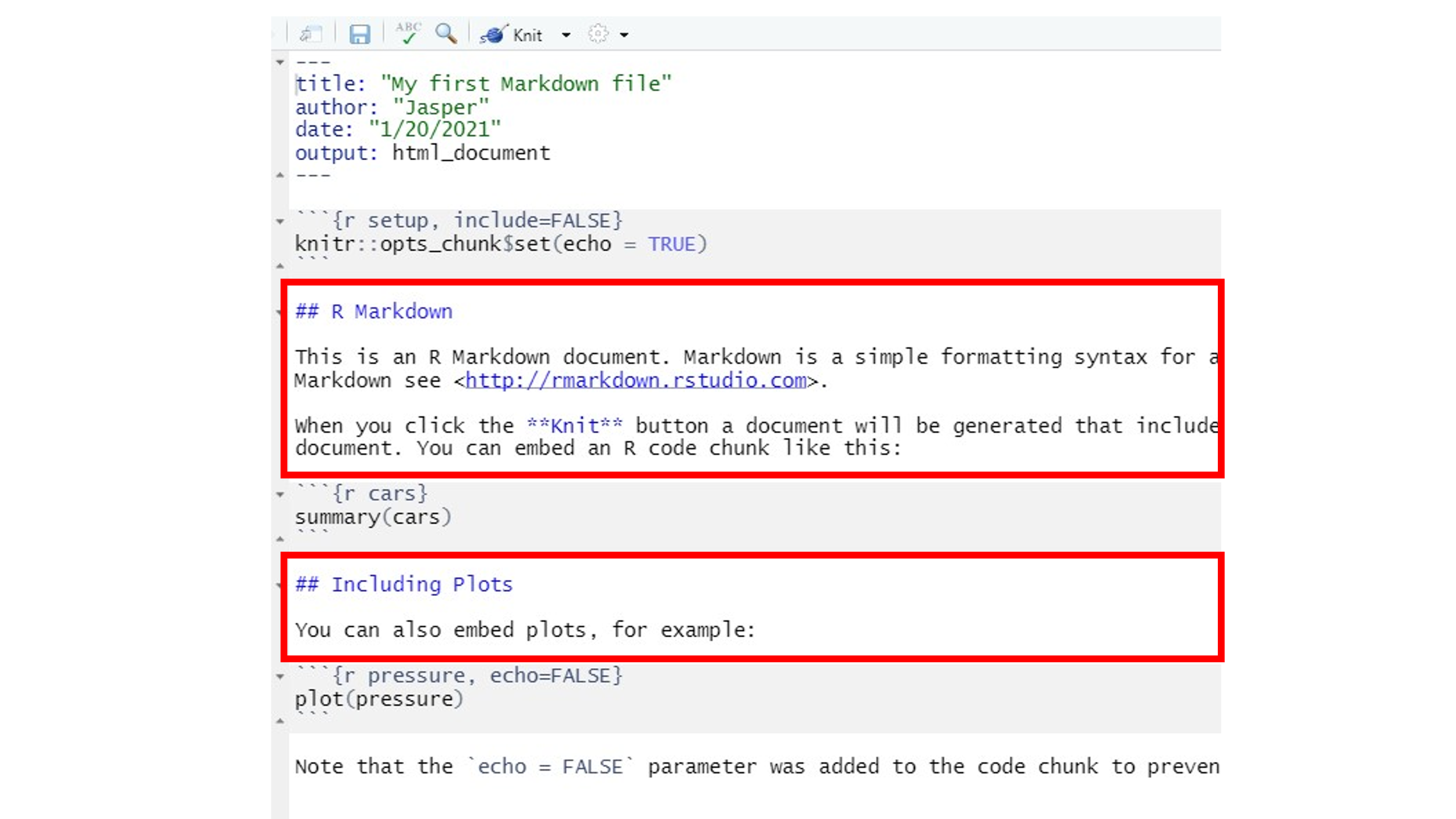
- Text: Narration formatted with Markdown. So this is just your
written text which you format using some tricks (more below). In the
picture,
#s indicate headings. The number of hash symbols represents the level and the font size of the heading. One big advantage of R Markdown in comparison to regular text editors is that you can still reference items from your analysis in the code chunks within your text. This means that when, for example, you want to state a number from your analysis within the text, you can just call it using inline code (which we will get to know a bit better later on) and it will automatically update whenever something changes. This way, you never have stressfully command-f-search your document to manually type and change a number every time something changes in your analysis. Cool, huh?
- Code chunks: The code chunks in grey always end and start with the
code delimiters
``` {...} and ```. It is between these code delimiters where the magic happens. Here we could do anything with R that we learned in all previous weeks. The arguments inside{}will define whether we want R to run the code (by including a simplerfirst thing in the brackets), whether we want to show the code in the final document, and whether want the outputs produced by the code (e.g. a Table or a Figure) to be displayed in the document. The first code chunk, for example, defines byinclude = FALSEthat neither the chunk nor its output is to be shown in the rendered output file. The argument in the last code chunk header isecho = FALSE, which will only display the output of a code chunk but not the actual code itself. Thus, we would get to see the plot in the rendered output file but not the code used, hereplot(pressure).
10.4.2 Knitting
Now, before we get our hands dirty with our first Markdown file, we need to address one more thing: Converting our zebra-style Markdown file to a pretty output file of our choice. Knitting is the R conversion process from the Rmarkdown file into the output document of our desire (in our case now, a html file). It is called Knitting because the conversion is done using the knitr package.
We should still have the default Rmarkdown file open (if not, go back up and check how we opened one). We can see the different parts described in the previous section. Now, let’s click the “knit” button on top next to the fitting icon of a needle in wool and as you will see, the html document will pop after you tell R where you want to save the file. Depending on your operating system, it may also just be saved in the same folder you are already working with. Also, don’t stress in case your pop-up window says “... file not found”: simply press the “open in browser” option on top and it should open in your default browser without a problem!
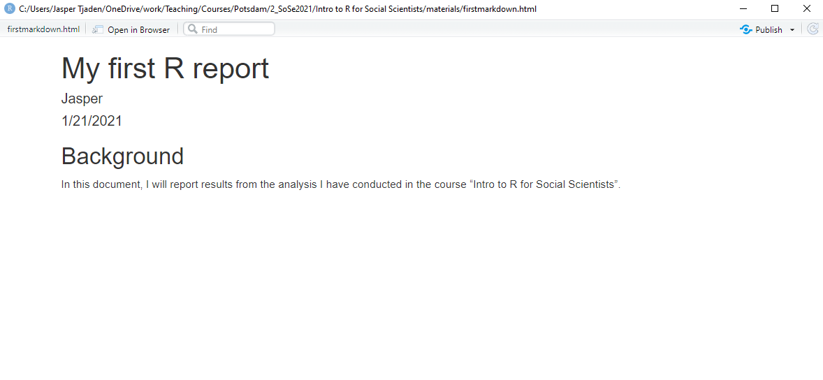
10.5 My first Markdown file
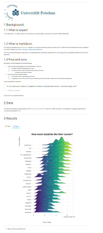
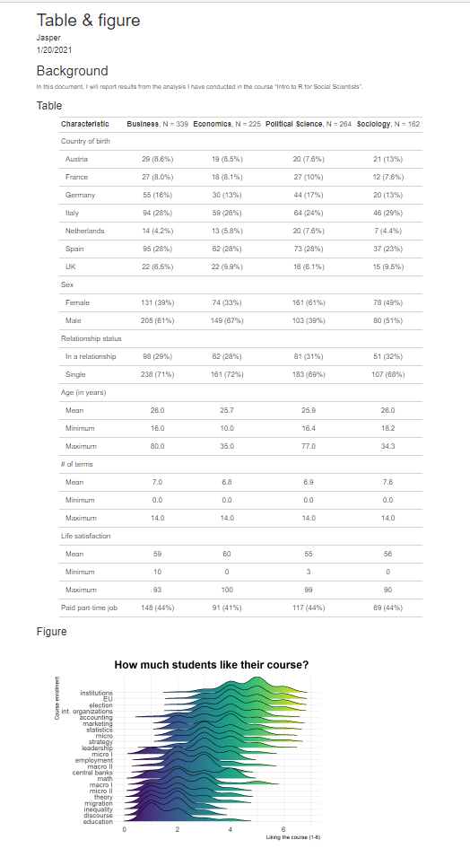
Now, let’s try Rmarkdown with our own data. Here is a screenshot of the final report we will produce.
Not too bad, not bad at all. Let’s go through step-by-step how we do this.
Step 1: Produce what you want to show in a R script
Remember the nice summary table we produced back in week 5 using the tbl_summary() function? Let’s find that code and paste it into a new R
script. Note: You could paste this code directly into the code chunk in
the Markdown to run it there. However, we will keep it separate in this
example. As we are starting from scratch, do not forget to install and
load all required packages and import the students dataset.
It should look like the code below and when you run the script, R will
produce the summary table in the plot output window on the right-hand
side. The table is saved as the object tab4.
Go ahead and save the R script under the name “week 9_rmarkdown_table.”
# clear all
rm(list = ls())

# load required packages (make sure they are already installed!)
library("tidyverse")
library("flextable")
library("stargazer")
library("janitor")
library("gtsummary")
library("writexl")
library("knitr")

# load all excel files
students <- readxl::read_excel("data/students.xlsx")

# convert variable types
students <- students %>%
  mutate(lifesat = as.numeric(lifesat),
        term = as.numeric(term))


# produce table

tab4 <- students %>%
  select(cob, sex, relationship, age, term, lifesat, job, faculty) %>%
  tbl_summary(missing= "no",
              by = c("faculty"),
              type = all_continuous() ~ "continuous2",
              statistic = all_continuous() ~ c("{mean}","{min}","{max}"),
              label = list(
                cob ~ "Country of birth",
                sex ~ "Sex",
                relationship ~ "Relationship status",
                age ~ "Age (in years)",
                term ~ "# of terms",
                lifesat ~ "Life satisfaction",
                job ~ "Paid part-time job"
              ))
tab4 | Characteristic | Business, N = 339 | Economics, N = 225 | Political Science, N = 264 | Sociology, N = 162 |
|---|---|---|---|---|
| Country of birth | ||||
| Austria | 29 (8.6%) | 19 (8.5%) | 20 (7.6%) | 21 (13%) |
| France | 27 (8.0%) | 18 (8.1%) | 27 (10%) | 12 (7.6%) |
| Germany | 55 (16%) | 30 (13%) | 44 (17%) | 20 (13%) |
| Italy | 94 (28%) | 59 (26%) | 64 (24%) | 46 (29%) |
| Netherlands | 14 (4.2%) | 13 (5.8%) | 20 (7.6%) | 7 (4.4%) |
| Spain | 95 (28%) | 62 (28%) | 73 (28%) | 37 (23%) |
| UK | 22 (6.5%) | 22 (9.9%) | 16 (6.1%) | 15 (9.5%) |
| Sex | ||||
| Female | 131 (39%) | 74 (33%) | 161 (61%) | 78 (49%) |
| Male | 205 (61%) | 149 (67%) | 103 (39%) | 80 (51%) |
| Relationship status | ||||
| In a relationship | 98 (29%) | 62 (28%) | 81 (31%) | 51 (32%) |
| Single | 238 (71%) | 161 (72%) | 183 (69%) | 107 (68%) |
| Age (in years) | ||||
| Mean | 26.0 | 25.7 | 25.9 | 26.0 |
| Minimum | 16.0 | 10.0 | 16.4 | 18.2 |
| Maximum | 80.0 | 35.0 | 77.0 | 34.3 |
| # of terms | ||||
| Mean | 7.0 | 6.8 | 6.9 | 7.6 |
| Minimum | 0.0 | 0.0 | 0.0 | 0.0 |
| Maximum | 14.0 | 14.0 | 14.0 | 14.0 |
| Life satisfaction | ||||
| Mean | 59 | 60 | 55 | 56 |
| Minimum | 10 | 0 | 3 | 0 |
| Maximum | 93 | 100 | 99 | 90 |
| Paid part-time job | 148 (44%) | 91 (41%) | 117 (44%) | 69 (44%) |
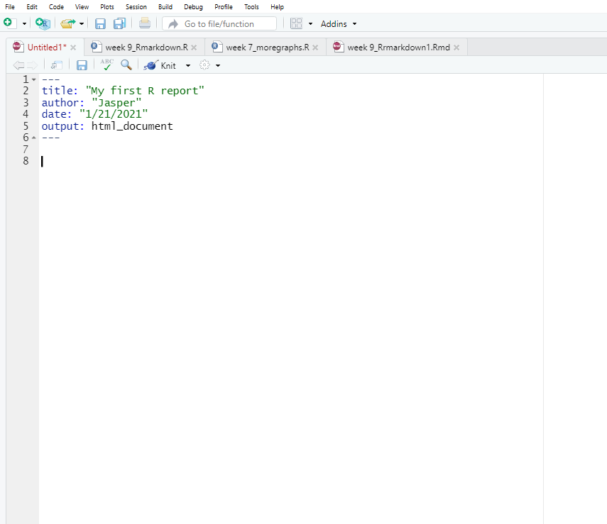
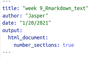
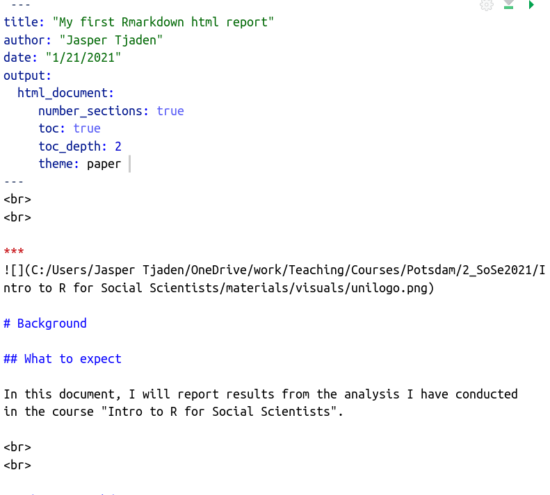
Step 2: Open new Rmarkdown file and delete everything you do not need
Go to File and open a new Rmarkdown file. The default template has things in it to show you how it is done. Delete everything except the YAML – the top part. It should now look like this:
Step 3: Write some text
Could be anything that you want in your report. For example, it could look like this:
Note that when you use a # sign, markdown will turn whatever is
followed by the hash symbol into a heading. “#” is a level one title
(large, bold), two “##” are a level 2 title (a little smaller) and so
forth.
Let’s assume we are done, and we want to export our document. Click the “knit” button, select a place where you want to save your html report, and then R will produce it. Mine looks like this now:
You are probably thinking what I am thinking: Not impressive at all, right? Very underwhelming. But let’s be patient. Step by step, we will turn this into a nicer report.
Step 4: Insert code chunk
You can insert an R code chunk either using the RStudio toolbar
(the Insert button) or the keyboard shortcut Ctrl/Strg + Alt + I (Cmd +
Option + I on macOS). This saves you some time (and nerves!) compared to typing ``` {r}``` manually every time.
There are a lot of things you can do in a code chunk: you can produce
text output, tables, or graphics. As mentioned above, you could run all
the code that produces our table here as well (we won’t do that). You
have fine control over all these output via chunk options, which can be
provided inside the curly braces (between {r }).
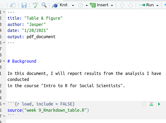
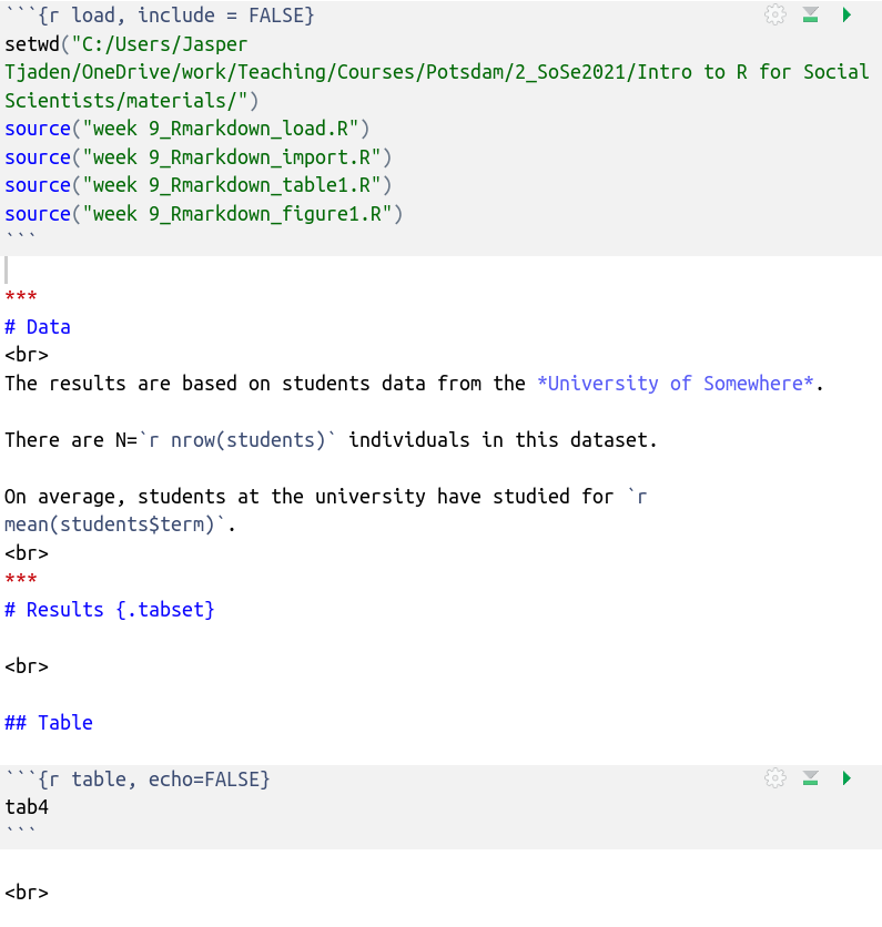
Let’s add a chunk. First, we need to name it. Give it a name that describes what the chunk is doing, but it should be one word.
Our first chunk will bring into Rmarkdown what we have done in the script. This is IMPORTANT: Rmarkdown is blind to anything that happens outside of it. Anything you want to include in the report, needs to be loaded inside the Rmarkdown file.
Since we want to show the table, we need to bring that output inside
Rmarkdown. To make that easier and to avoid repeating code, we can call
on saved scripts inside Rmarkdown using the source() function. When
we do that, Rmarkdown runs the entire script and loads all the outputs
included in that script. It also loads all loaded packages and imported
data specified in the script which enable you to produce the output in
the first place.
Have a look at this first code chunk below.
Any code chunk starts with ``` {...} and ends with```. The first
line has the {} brackets. In it we have “r” and the name we assigned to
the code chunk “load” (because I want to load our analysis). Be careful,
each code chunk needs a unique name! But also, you don’t have to add a
name.
Inside the chunk, we are telling R where to find the script by setting
our work directory using setwd() and then use the source() to
run the script. Try knitting the doc. As you can see, nothing changed
that our eye could see.
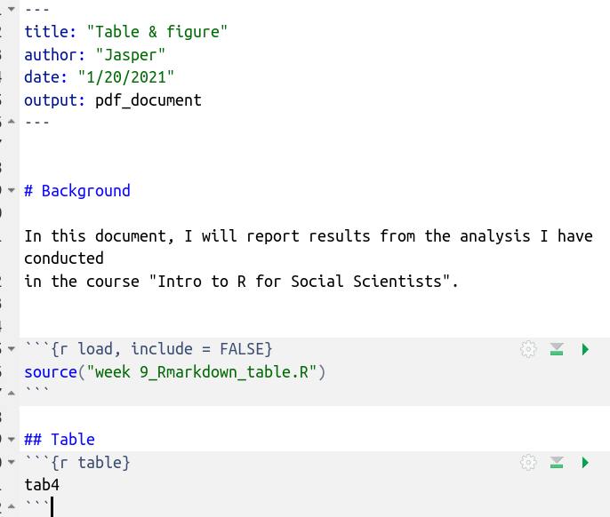
Now we that we have the data and the analysis loaded, let’s include the table. First, we create a new code chunk and give it the name “table.”
There are always two parts in a code chunk: the code itself, followed by
the output generated by that very code. The options “echo,” “include,”
“results” are all meant to specify whether you want to show 1) only the
code 2) only the output or 3) both. See
here for more chunk
arguments. Note the first code chunk option here: include=FALSE. As a quick reminder, the
“include” options specifies whether we want to actually show anything
that is happening inside the code chunk in the report while still
running it. We select FALSE because our audience does not want to see
our code. The “echo” option specifies whether we want to show the reader
the source code above the created output or just the output (the table).
We selected echo=FALSE for the second code chunk with the table
because we want exactly that: only the table output, not the code. Inside
the code chunk we just call on the object tab4 which is the name we gave
the table we created in the R script we just loaded into our Rmarkdown
file.
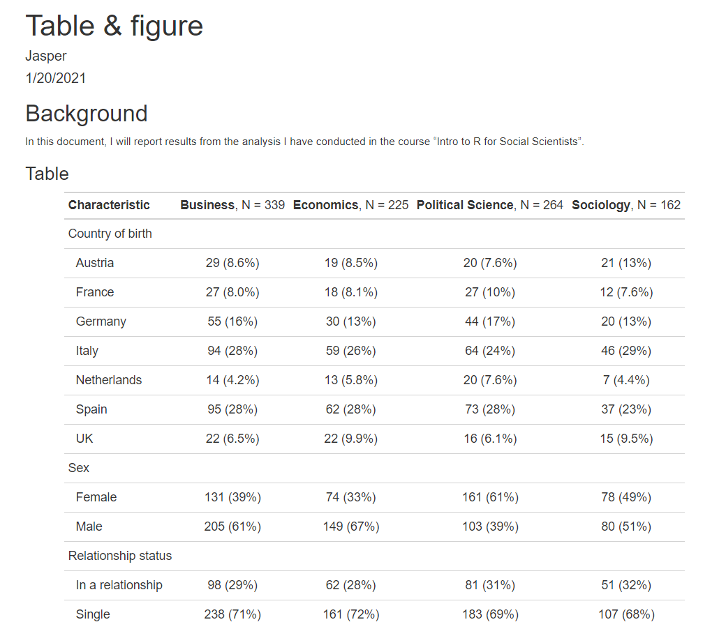
Note: I also added the word “Table” above the code chunk as text. Now let’s knit this.
We are getting there. The Table is included.
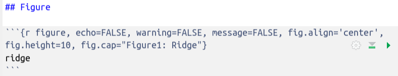
Now, let’s include a figure as well. We need to run through all the steps I outlined above. I will not go through each step again, but rather show you the final output.
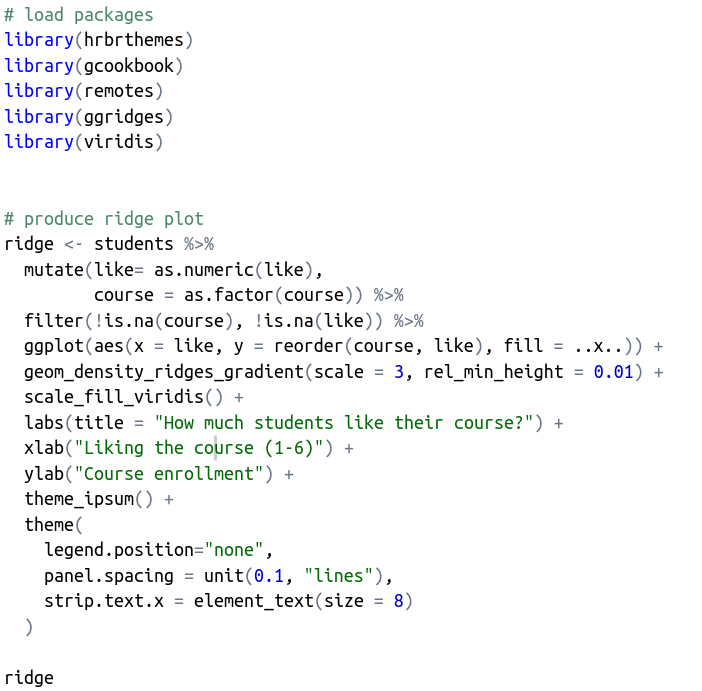
Remember this nice ridge plot which we produced in week 7? Let’s include this one. Save a script that produces the plot. Alternatively, just run the script you had for that week. It should look like the below. Don’t forget to install and load all required packages if you have not done so already.
Our ridge plot is saved as the object “ridge.” Save the script, for example as “week9_rmarkdown_figure.”
Now, reference the new script in the Markdown file.
Tip: Notice that when you only run one code chunk by either selecting the code chunk or clicking the green little arrow on the side of the code chunk, that the objects generated by the code pop up in the environment (upper right-hand panel).
Also notice that there are two new code chunk options: warning=FALSE
and message=FALSE. These options tell markdown not to include any
type of message or error warning produced by the code. Try knitting the
doc without these options and you will see what I mean.
Here we are: We have our first report:
10.6 Workflow & Organization
10.6.1 Multiple Files
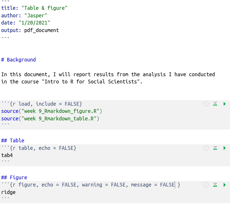
Note that in our example above, we are running two separate scripts
using the source() function:
source("week 9_rmarkdown_table.R")
source("week 9_rmarkdown_figure.R")
Remember how the first script produced the table? It first loads a bunch of packages, then imports the data, cleans it a little bit and lastly, produces a table. The second script loads some packages and then only produces a figure using the same data that was imported in the first script. This can get messy if your analysis gets very long and you are using many scripts that are all building on each other.
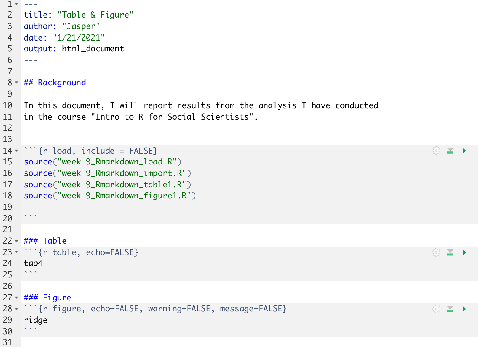
I recommend keeping different steps of the analysis in different
scripts. For example, in our case, I would have separate scripts to
install and load packages, to import and clean the data and to apply all
kinds of analyses and manipulations for output generation. If we later
need to change something, we know exactly where to go instead of
checking all scripts and figuring out how they relate to each other.
Each script can work on its own. Recall that since Rmarkdown runs all
the scripts it calls one after the other, all the packages and data
loaded in a previously loaded script are available to the following
(except, of course, you choose to clear your workspace using rm(list = ls()) in the meantime). This allows you to have separate scripts for
loading packages, data etc. and frees you from having to load all of it
in the beginning of every single script you include.
If we reorganize our scripts, it would look like the image below. Note that we now split the analysis into clean separate scripts.
The more complex a project gets, the more steps involved, the more people involved, the more you need to think about workflow: Who does what when and how does it feed into another step in the chain? In our case, for now, let’s assume we work alone. We want to produce an annual report that pulls together all the analysis bits we have produced over recent months.
There are two different general approaches to organizing your workflow when using Rmarkdown:
All-in-One: You only use Rmarkdown files and do your data management and analysis there. The clear advantage is that you only have one file for everything. As we have seen there are ways to hide steps in the analysis that you don’t want to include in the report.
2-Step: You prepare your analysis in R scripts (as we have done in all previous weeks), you save your outputs (tables, graphs etc) as an object, then you use the Rmarkdown file only to output the saved object results that you want to show in the right order (adding text if you want).
What is better? This is up to debate. As far as I can tell, there is no clear answer. It depends somewhat on the preference of the analyst. However, you might want to stick to the second approach if the analysis includes very different kinds of steps, such as web scraping, topic-modelling and data analysis.
The 2-step approach that I have introduced you to has one main advantage. The order in which you do your analysis and produce different results does not matter. You produce them somewhere, save it and then call them later. If you separate the code producing the analysis from the code reporting it, it is easier to keep track of your actions and outputs. In my view, it is a little cleaner. You can divide various steps of the analysis into different R scripts.
For example, maybe you have one script producing one complicated table. It takes 40 lines of code as you first must change the data for the table. You save it as “Table1.” In the Rmarkdown file, you do not worry about the data, the cleaning and how the table was produced. You call on the script and just use the end product “Table1.” If you need to change the table, you do not have to make changes somewhere in the Markdown file. You simply go to the relevant script and change it there. This leaves the Rmarkdown file clean and easy to follow. If you do data wrangling, data manipulation and data generation in the Rmarkdown file, the file can get very long and hard to follow.
10.6.2 R Projects
Another way to organize your work are R Projects. It simplifies working with multiple files in multiple locations/ directories. It makes setting the directory easy and helps files to refer to each other.
You can start a project by clicking on “File” -> “New project.” You will then be asked for a location on your computer where you want to put the project. R will then create a folder. Now, all scripts that you will be using for this project will be saved automatically within this environment. You do not have to manually indicate the location anymore when you open the project file.
When you open the project file, you will see all files associated with the project in the buttom right corner in the “files” tab in R Studio.
As you projects get bigger and more complex, organization becomes ever more important.
10.6.3 Working in teams
Throughout this course you have worked alone with your dataset. In today’s world, this is increasingly uncommon. Tasks get more complex and involve several analysts working in teams. While working in teams is fun and (in the ideal case) can save time, it also brings with it some organizational challenges when team members work on the same file at the same time.
One approach is to use Google Docs, Google Sheets or Microsoft sharepoint. All these applications host files on clouds and allow users to work on files simultaneously.
For us data analysts, common cloud solutions are not ideal because they are not made for writing code. The go-to solution is GitHub, a code hosting platform that allows linking repositories with all the files you want to (collectively) work on with your own computer.
It offers the distributed version control and source code management (SCM) functionality of Git (a version control system), plus its own features. It provides access control and several collaboration features such as bug tracking, feature requests, task management, continuous integration and wikis for every project.
Along with the creation of a project goes the creation of a GitHub repository (repo), an online directory or storage space for your project. In order to start collaborating on a project, collaborators have to clone the project. The main basic features are fetching, pulling, committing and pushing.
Before introducing any changes to the project, it is advisable to first check whether the version of the project on your local machine corresponds to the remote version on GitHub. In other words, use fetch to check the remote version for updates. If there are changes to the remote version that do not exist on your local version, you can pull these changes to your local machine, i.e. update your version on your local computer. The subsequent pull is going to be reflected in the updated files in your project folder.
After each big change, it is recommended to save your progress via commit and to note down your changes with a concise description. Thereby, it is easier for you to go back in time to retrieve an older version or revert changes. As soon as you are ready to update the remote version on GitHub and share your progress with your collaborators, overwrite the remote version via push. In other words, push your changes to the main/master version.
Git makes it easy to compare the changes made in different versions and to reconcile/merge them. Another big plus is that you can easily go back to older versions if something went wrong.
To find out more about Git and how to use it go here, here and here.
Click here for a selection of Git GUI Clients, i.e. nice graphical user interfaces for managing Git. Unless you prefer operating Git via your terminal.
GitHub also allows you to host websites that you can create with R blogdown.
This whole course was developed and launched using bookdown in combination with GitHub Pages.
10.7 Fine tuning
There is literally nothing you cannot change in a Rmarkdown file. The problem is that it can get quite complicated quickly and there are many ways to achieve the same goal. Here is a good resource on “customizing” markdown files.
In the following, I will cover simple and basic approaches to:
How to format your text?
How to format the tables and figures?
How to change the overall look and structure of the whole file?
As always, I will try to provide additional resources through hyperlinks.
10.7.1 Formatting text
We have been working with a Rmarkdown file. Make sure to save it in your directory. Now, I will run you through a file where I included more text to show you some of the formatting options. For more guidance on formatting, click here as well.
10.7.1.1 Sub-sections
There are three levels for headings. Use “#” for the first, “##” for the second and “###” for the third. Make sure there is a space after the # sign. Again, compare the sample code with the knitted output.
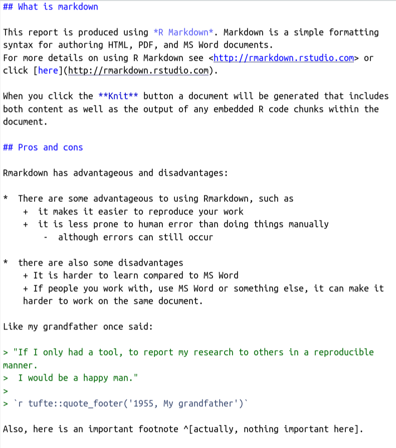
10.7.1.2 Bold and cursive
If you want to make a word or sentence appear in cursive, embrace it with single stars like *…*. If you want to make it bold, use double stars **…**. Look at the second and third paragraph in our example: “R markdown” is cursive, “knit” is bold.
10.7.1.3 Highlighting
You can highlight text by writing <mark>…</mark> around the part that you like to have highlighted.
10.7.1.4 Empty rows/ paragraphs
Notice that there is more space after the first paragraph. I simply added two empty rows. You can do that using “<br/>.”
10.7.1.5 Hyperlinks
To link to a website in your document, you can either state the internet
address (URL) and enclose it with the <…> signs. Then the URL itself
will appear as a hyperlink. If you want the hyperlink to be attached to
another word (the label), then type the label enclosed by brackets as in
[label], followed by the URL enclosed by parentheses. No space in
between. Have a look at the code and see how it looks when you knit it.
10.7.1.6 Lists/ bullets
Use “*,” “+” and “-” for bullets and dashes in lists. Make sure each sub-level is 2 tabs to the right. Also, make sure there is an empty line preceding the first level. See how I did it here:
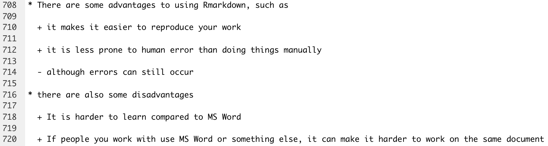
There are some advantages to using Rmarkdown, such as
it makes it easier to reproduce your work
it is less prone to human error than doing things manually
although errors can still occur
there are also some disadvantages
It is harder to learn compared to MS Word
If people you work with use MS Word or something else, it can make it harder to work on the same document
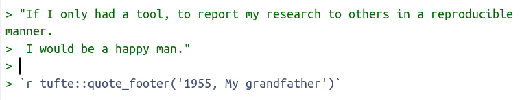
10.7.1.7 Quotes
To include quotes, use the > greater-than-sign in front of every quote line to put it into block format. Include quotation marks. You can also include the author using the tufte package. Load and install it in the loading script, e.g. “week9_Rmarkdown_load.R.” Save the script and add the content below to your markdown file.
10.7.1.8 Footnote
You can add footnotes with the “^” wedge symbol immediately followed by
what you want to put in the footnote in square brackets [...].
10.7.1.9 Inline code
A key motivation for knitr is reproducible research: we provide the data and the code which we used to arrive at our results, rendering our results more trustworthy and facilitating reproducibility and progress.
Thus, your report should never explicitly include numbers that are derived from the data. They could change. Don’t write “There are 168 individuals.” Rather, insert a bit of code that, when executed, returns the number of individuals.
That’s the point of the in-line code. You can reference a number from
your data in the text typing r followed by three dots. For example, take a look at the
data section in the report. We tell the reader how many students are in
our dataset by calling the nrow() function on our dataframe.
You’d write something like this:
There are N = nrow(students) individuals in this dataset.
Another example:
The estimated correlation between x and y was cor(x,y).
In R Markdown, in-line code is indicated with r and apostrophes. The bit of R code between them is evaluated and the result inserted.
If you want to reference specific number like the average life satisfaction in the text somewhere. Save that number as an object and then call it in the text.
10.7.2 Adding images
You can add any image to your report. I added the logo of the University
of Potsdam. First, you need to save the image file (.jpeg or .png) in
your local folder. The you use ![] to include it followed by the
location of the file in parentheses.

More on fine-tuning images go here.
10.7.3 Formatting output/ code chunks
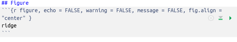
10.7.4 Alignment
Let’s say we don’t like that our ridge plot is “left-aligned.” We want
it in the center. We can change that in the code chunk option using
fig.align=.... In our case, let’s use center.
10.7.5 Size of the output
You can use fig.width and fig.height in the code chuck to change
the figure size. Try it out, individually one after the other,
fig.width=5 and fig.width= 15, fig.height=5 and
fig.height=15.
With fig.dim = c(5,5) you can change both width and height at
once.=15`.
If you are dealing with images and not output generated in R, you can use out.width and out.height.
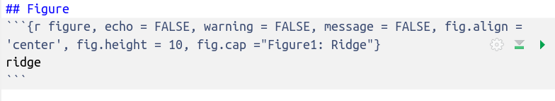
10.7.6 Adding captions
You can add a caption for the graph by using fig.cap =. Let’s do
that for our ridge figure. Note that this approach only works for
figures produced using ggplot.
10.7.7 Formatting the structure of the whole argument
10.7.7.1 Add numbering
Markdown can automatically number your headers on each level. To do this
you need to add the number_sections: true argument in the YAML
header. See here:
You can also add numbering manually, simply by typing out the number as text: “1. Header” etc.
10.7.7.2 Tabs
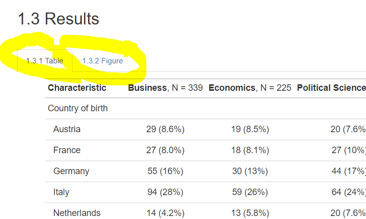
Rather than structuring your report in the traditional top to bottom approach with different headings, section-headings and sub-section heading, you can organize different parts of your file in so-called tabs, that is, sections.
Let’s try this out and put the table and figure in separate using {.tabset}. Write {.tabset} after the heading that preceeds the section that you want to appear in tabs. R will then automatically put any lower
level in a tab.
So when I place {.tabset} after ## results, like this:

Then the next section will be grouped in tabs, like this:
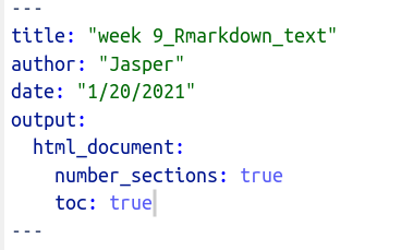
10.7.7.3 Adding table of content
Some reports include “Table of contents” (toc). Let’s include one in our report. Just add “toc: true” to the YAML header, just like we did for the numbering. Make sure it is indented by one tab. The Table of Content is automatically hyperlinked to the various sections in our report.
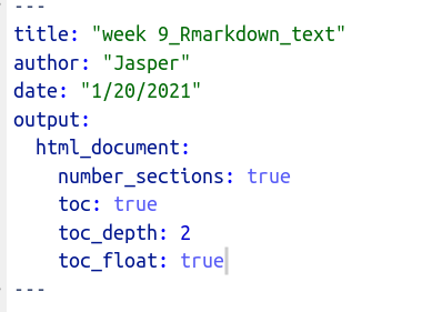
Also, you can change how many levels you would like to include in the
toc using toc_depth:.
If you would like to switch the toc to the side, and not have it above
the report, you can use toc_float=true:
10.7.7.4 Changing the look: themes
During this whole lesson, we have explored how to fine-tune and change different elements in the markdown report. You need these basic skills to adapt any markdown report. Admittedly, however, the report does not look very “beautiful.” I may have convinced you that Rmarkdown is good for reproducibility and adds a lot of functionality in html reports, but if it is ugly, we may not consider it. In the end MS word is just easier to adjust the look.
Hold on.
“Themes” are one way to change the overall look of your document with one line of code. Be assured that you can also change any aspect of your report manually, however, it gets complicated and requires knowledge of Markdown language.
Here is a
list of standard themes that come automatically with Rmarkdown. And this
list grows by every year as people (don’t ask me who has the time to
develop these themes, but I am grateful) develop and submit new themes.
For example, the package
rticles includes many themes
for particular academic journals. These themes apply an overall layout
on the whole document, including specified font size, font, colour
scheme etc.
We won’t get into all that. For now, we will just apply a standard
theme. Let’s take the “paper” theme and apply it to the document by
adding theme: paper in the YAML. Looks much better already, right?
10.8 Summary
We have added elements step-by-step. For reference, here is the whole Rmarkdown file:
10.9 Exporting to Word
HTML output is great to design reports, make them reproducible and to
add some interactive elements to your report. For example, we have put
certain sections in tabs, so reader can select the outputs they would
like to see. There are many more ways to make things interactive that we
have not covered yet, including making plots interactive (see
plotly(), ggiraph(), leaflet()). Html reports are the option
of choice for those type of reports. You can also turn html reports into
website or embed them in one which can be very useful.
However, there are sometimes scenarios where you cannot – or I should say – are not supposed to use html reports. This can be the case when 1) the degree of customization exceeds your markdown enthusiasm or 2) you work in collaborative projects with others who do not use markdown.
I have been in both scenarios. Some reports need so much tweaking and detailed features that I don’t want to invest the time in properly learning the underlying languages (e.g markdown, html, css etc.). Second, many of my projects were collaborative. Several people were working on the same document, drafting, reviewing and editing various sections together. MS word is great for that: you can leave track changes, comments and compare versions. You could do some of that in Markdown but we are still far away from MS Word’s intuitive usability and universal reach.
So, what do we do?
Good news: Rmarkdown can export your results to MS Word.
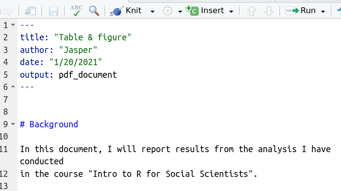
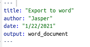
Remember when we first opened our new Rmarkdown file? Let’s do that
again but instead of selecting “html,” let’s select “word_document.” Also, delete
all the default stuff R automatically puts in our file. It should look
like below. As you can see, so far, the only thing that changed is the
output: word_document
Now, just insert our code from the previous .Rmd file into the new one. Then, knit it. You will see that R now produces a word file. It is possible to change the formatting beforehand using a reference document (see explainer video here), but we won’t do that now.
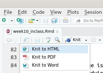
Alternatively, you could also just click on “Knit to Word” under the drop-down menu of your “Knit” button instead of directly directly hitting the “Knit” button in your Rstudio.
So the general strategy would be that you produce the entire report in MS Word, and only produce the analysis in R. Then you export the tables and figures to MS Word and move them into another doc.
10.10 Common issues
Rmarkdown offers amazing functionality. It looks pretty easy, but I have chosen examples that were straight forward. I made sure beforehand that they will work. Rmarkdown can be a “rabbit hole” in which to get lost and despair. Here I want to list some of the most common issues and their solutions:
- Packages not installed and loaded at all or at the right time
This does not just apply to markdown, but to R more generally. However, it is more confusing when adding .rmd files because they reference other R scripts. Somewhere down in your rmd file, you may be running a function that has not been installed. I recommended using one dedicated script to install and load packages. However, it then becomes difficult to remember which package does what. When you get an error, R will tell you which package is missing. Go back to the loading file and add it.
- Workflow messed up
When your analyses get larger and longer, your files will expand. Organization and structure become very important. Remember that we always want our analysis to be reproducible. You should always feel confident to send your code to someone else for them to run through it without a problem. Implement different steps in your analysis in different files. Use concise names and always comment in the files to remind your future self and your collages what you were trying to do. Rmarkdown produces errors when you are trying to do something that has happened outside the .rmd file. Make sure you reference all steps at the right time.
- Type of output not suitable for markdown code
Exporting results from R is not super straightforward. Some types of output formats are not compatible with certain export formats. You may produce a kind of table object that won’t render in the html file. Or you may produce a table object that isn’t compatible with MS Word. Always make sure you are aware of which type of object you are storing results in (by using the help() function and looking up the relevant function).
- Think hard beforehand what kind of report you want
Think hard before you start what the requirements are for your report. It will influence how you organize your work, when and how you do things. For example, if you know you want to export your results to Word, you could leave out the titles for figures in R and then add them manually later in MS Word. If you know you are exporting to word, you won’t have to invest any time and thinking into how to make things interactive, for example. When you want to produce a fancy report as a html file, make sure that your supervisor doesn’t ask you later for the possibility to comment in Word.
10.11 Exercises I (based on class data)
Last week, you truly knocked your employer and the Board of Education off their socks. No, really! But you feel like adding yet another cherry on top! So far, you’ve always copy-pasted your code outputs to a Word document. Now it’s time to do both the output generation and the output report in Rstudio!
Go back to the last weeks and get the code for one of the summary tables (week 5) and the line-graph from week 6. Save them in separate R scripts and name them meaningfully. Now, load them in your Rmarkdown file.
Add concise descriptions of the table and the figure with 2 sentences to each illustration answering to questions: What does the illustration show and what finding is of particular interest? Also make use of stylistic devices such as bold or cursive highlight.
Tell the reader how many students were in your dataset using in-line code
Add a third output and arrange all three in different, horizontal tabs. Let’s choose the first violin plot from week 6.
The report should be pleasing to the eye, so we picked some images from the internet to append them to the figure and the table. However, please do add the source of the image as a hyperlink. The images can be found here and here.
Lastly, select a theme of your choice. But do not pick the one used above.
Deliver the results in both a HTML and WORD format.
10.12 Exercises II (based on your own data)
Similar to above, please pick one graph and one table you’ve produced in the previous weeks and display it in a converted Rmarkdown file. Feel free to choose the format.
Add a concise description, an image as well as the sources of the image to each output.
Select a theme that was neither used by the instructor nor by you in class.