12 Week 12: Mock Exam
12.1 Introduction
You have almost made it! Before finishing the course, you can now apply what you have learned to a new dataset.
You should set aside three hours to complete this exam. It is an “open-book” exam, so don’t hesitate to look up things online or in the class materials. Of course, the more you need to look up, the less time you will have to complete all tasks.
12.2 Grading
As orientation, I have indicated the points I would give for each exercise. In total, there are 85 points. 79 are for correct answers to the exercises, 6 points are given for 1) clear and replicable code and 2) efficient/ sophisticated code.
| Grade | Points |
|---|---|
| 1.0 | >80 points |
| 1.3 | >75 |
| 1.7 | >70 |
| 2.0 | >65 |
| 2.3 | >60 |
| 2.7 | >55 |
| 3.0 | >50 |
| 3.3 | >45 |
| 3.6 | >40 |
| 4.0 | ≥35 |
| Fail | <35 |
12.3 Scenario
Your friend calls you and starts asking about your R journey. They are curious to hear how much you were able to learn in such a short amount of time – and end up pretty impressed! By now, you are already quite familiar with people requesting your skills to help them with some urgent project and you have a feeling where this conversation might be going.
Instead, your friend wants to know when you will start with that passion-project of yours that you kept postponing for your various side hustles. So for a change, you decide to have a closer look at some data you are interested in yourself: the European Social Survey!
12.4 The Dataset
The European Social Survey (ESS) is a cross-national survey that has been conducted across Europe since its establishment in 2001. Every two years, face-to-face interviews are conducted with newly selected, cross-sectional samples. The questions focus on attitudes, beliefs and behaviour patterns of diverse populations in more than thirty European nations.
Here is the list of columns/ variables included in the dataset provided for the exam: Make sure to have a good look at the list because you will need to come back to it for most exercises to identify the information you need to complete the tasks.
| Variable | Explanation |
|---|---|
| essround | round of the European Social Survey (here: 9) |
| cntry | Country where survey was taken |
| marsts | legal marital status |
| eduyrs | years of full-time education completed |
| mnactic | main activity during the last 7 days before the interview (work?) |
| hinctnta | household total net income (decile) |
| netusoft | internet use frequency |
| ppltrst | generally speaking, can most people be trusted? |
| vote | voted in the last election |
| prtv… | party voted for in last election, suffix according to country (…at, …de etc.) |
| contplt | contacted politician or government official last 12 months |
| wrkprty | worked in political party or action group in last 12 months |
| sgnptit | signed petition in last 12 months |
| pbldmn | participated in lawful demonstration in last 12 months |
| pstplonl | posted or shared anything political online in last 12 months |
| lrscale | political standing, placement on left-right scale |
| agea | age of respondent (calculated) |
| wkhct | working hours contracted, overtime not included |
| EU_… | European unification go further or gone too far |
Let’s get started!
12.5 Exercise 1: Getting Started (12 points)
First things first, you need to load everything you need. Lucky for you,
someone already put together the files for Austria’s, Denmark’s,
France’s, Germany’s and the Netherlands’ Wave 9 survey data and saved
them as ESS_data.RData1. The data can be found here.
Open the help-file for the
load()command and then apply it accordingly to the dataset. Hint: No need to assign it to a name here, it will simply appear asESS_datain your environment! Make sure you tell R where the data is located and load all required packages. (1 point)Keep only the variables essround, cntry, ppltrst, lrscale, agea, vote, eduyrs, mnactic, wkhct, netusoft, pstplonl, contplt, sgnptit, and the party vote variables prtvtddk, prtvtdfr, prtvede1 and prtvtgnl. Kick out everyone from Austria. (2 points)
Your first encounter with the new data calls for some exploration.
Use a command to get an overview of the dataset, which variables are included and what types they are. How many variables in the dataset are “numeric” type variables before any recoding? (2 points)
Check in how many countries the survey was taken. How many people participated in the survey in the Netherlands? (1 point)
You decide to spell out all the country names which are currently abbreviated. Check whether the recoding worked. (1 point)
Check two variables representing “people’s trust” and their “political standing” and see 1) what type of variable they are and 2) quickly generate a univariate frequency table for each variable to see how the variables are coded and distributed. (2 points)
Convert both variables in d) into a numerical variable on a scale and recode individual values. Hint: Make sure to match the answers perfectly, e.g. copy the right apostrophe! (1 point)
Have a closer look at the remaining numerical variables in the dataset and check whether their missing observations are handled appropriately and adjust if needed. Values like -99 and -999 should be recognized by R not as numbers but as missing values. Hint:
NA_real_may come in handy here! (2 points)
12.6 Exercise 2: Summarizing (8 points)
Phew, that was a tedious start. But now, you can finally start and have a look at the actual – and now nicely cleaned – data! You begin with some summary values:
How many people who have answered the survey have voted in the last election? (1 point)
What is the average number of years spent in education per country? (1 point)
What is the percentage of Danish survey respondents who are retired (hint: check the activity of respondents during the last 7 days before the interview)? (2 points)
How many people work at least 30 hours a week (contractually)? (2 points)
Is the share of survey respondents working at least 30h per week higher in Germany or in the Netherlands? (2 points)
12.7 Exercise 3: Producing Tables (10 points)
You know more about your data now so you think it is time to produce some output so that you can show others what you are learning from the data!
For your first Table output, you choose to compare internet usage frequency of respondents with whether they posted something political online in the past year. Produce a table and save it as an object. Use a package of your choice! (Note: extra points for nice labels for variables and overall look). Are people that are online every day more likely to post something online than not? (4 points)
For your second output, you decide to create a summary table where you display the age of respondents, contracted working hours, trust in people, and whether they have shared political content online in the past 12 months by country. Make sure to report means for numerical variables and percentages for categorical variables, include minimum and maximum values for continuous variables) (6 points).
12.8 Exercise 4: Visualization I (6 points)
You are quite happy with your tables, so you decide to get a bit creative with visualizations. Your first plot is a violin plot displaying the age distribution of respondents by country. Make your plot pretty and easily understandable (i.e. labelled)!
12.9 Exercise 5: Visualization II (10 points)
Great, this looks very presentable! Next up, you find an interesting plot (see below) and decide to replicate it. Let’s go!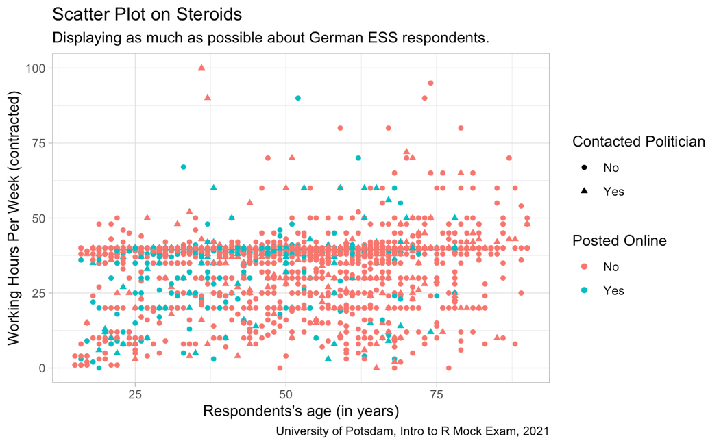
12.10 Exercise 6: More Data (6 points)
Amazing progress so far! It occurs to you that only looking at four countries can be quite limiting. You decide to add data from the European Social Survey on Belgium (Wave 9).
In order to do so, you visit the webpage linked above and register with your (university) mail address. When asked for a reason for your query, normally stating “seminar,” “exam,” “uni research” or something similar should be sufficient. Access the Wave 9 data set for Belgium and download it as a Stata file.
Now, you have to figure out how to load a Stata (.dta) file into R. The relevant file is called “ESS9BE.dta.” The “foreign” package is a good place to start. Hint: Use
help(package=foreign)to find the appropriate command to import .dta files into R using the “foreign” package! (4 Points)You proceed using the newly imported data. In case this did not work out, please proceed using the provided file “belgium.xlsx” (no point loss in this part of the task!). The Belgium file has far more variables than the previously used “ESS_data.” You are only interested in the variables regarding the last election (vote and country-specific voted for party) besides the country and round. Drop all remaining columns and then bind the two dataframes together. You can find the variable name for Belgium’s last party vote on the webpage under ESS > Data and Documentation by Theme > Politics > Data/Variables Round 9 (2018).(2 Points)
12.11 Exercise 7: Mapping (12 points)
You want to create a map with the newly extended ESS data. This map should show the share of voters as well as the party receiving the most votes among respondents per country.
For this exercise, proceed with the data frame you have, no matter whether Belgium is included or not! You go ahead and create a dataset containing only the country names and the share of respondents in each country who voted in the last election.
To this dataset, you add the party with the most votes among respondents for each country.
In the next step, you begin preparing the actual map by defining which countries you want to display, getting the respective map data and merging this data with the dataframe constructed in the step before. Each country is filled according to its respective vote share and the name of the party with the most votes among respondents is displayed in the middle of each country.
12.12 Exercise 8: Integrating into RMarkdown (10 points)
Pretty excited about your new plots and tables, you want to all put them together in one report. Integrate one table, one figure and the map into Rmarkdown. Describe each output in one sentence. Make sure to load everything! (7 Points)
Display the table and figure in tabs and include a table of content in the RMarkdown document! (3 Points)
12.13 Exercise 9: Reshaping (5 Points)
There is one more topic you are interested in: respondents’ attitudes towards European unification! You decide to have a look at the file “ESS_eu.RData” (which can be found here): Respondents were asked to specifiy their attitude between “Unification already gone too far” (0) and “Unification go further” (10). The data frame includes the average score per country in the ESS survey rounds 7, 8 and 9.
Load the data and explore the reshaping commands
pivot_longer()andpivot_wider()to refreshen your memory. Convert “ESS_eu” from wide to long and get mean values per country. What is the average score in Denmark (DK)? (3 Points)Convert “ESS_eu” from wide to long again but this time get the mean values per ESS round. What was the average score in the ESS round 8? Convert the long data frame with the mean values back into wide format. (2 Points)
Data Source: ESS Round 9: European Social Survey Round 9 Data (2018). Data file edition 3.0. NSD - Norwegian Centre for Research Data, Norway – Data Archive and distributor of ESS data for ESS ERIC. doi:10.21338/NSD-ESS9-2018.
Accumulated Data: European Social Survey Cumulative File, ESS 1-9 (2020). Data file edition 1.1. NSD - Norwegian Centre for Research Data, Norway - Data Archive and distributor of ESS data for ESS ERIC.↩︎