4 Week 4: Data Management II
4.1 Combining and Restructuring Data
Objective of this session:
Learn how to combine different datasets into one.
Learn how to change the structure of your dataset to be able to run different types of analyses.
R commands covered in this session:
merge()
bind_rows
pivot_wider()
pivot_longer()
unique()
distinct()
4.2 Combining Data
At times, the data you need in order to run your analysis or create a beautiful graph is scattered across different datasets. One key skill of any data analyst is to bring different datasets together. This process is commonly referred to as “merging” or “linking.” This task is crucial to get right and most jobs dealing with data will require this skill regularly.
In our case, for example, we have a dataset on students at the university. But we also have a separate dataset on courses offered at the university and another dataset on the four faculties where students are enrolled. Imagine you are interested in whether the timing of a class (early morning or late evening) has an influence on the average grades of students and whether this is different across different faculties. To answer this question, we need to first integrate information from all three datasets into one.
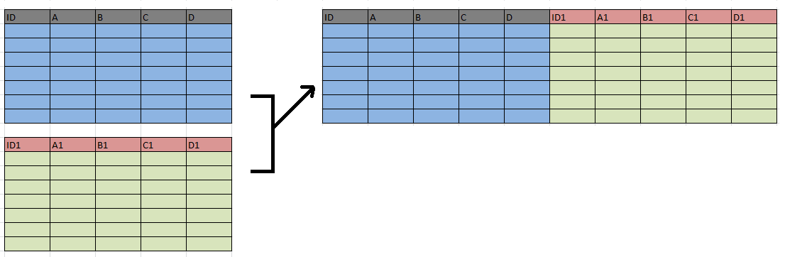
There are two ways to combine data: You either combine columns or your combine rows.
Combining columns: To do this, you need what is called an id or key
variable, i.e. some information that is identical in both datasets and
unique in at least one of them. For example, if you want to combine data
on courses with data on students. The student dataset needs to include a
variable on the courses of each student. We also need the info in the
course dataset to be unique, meaning that we only have one row per
course. You can merge (sometimes also called “match”) data either 1:1
(e.g. linking each student across datasets) or 1:many (linking many
students to courses that several students attend). R does most of that
automatically. The last step is deciding which combinations of data you
want to keep.
Merging
Combining rows: Combining rows is often called “appending.” Imagine you get new student data every term and they all arrive in separate excel files. You need to add them together for analysis. One important requirement is that (at least some) columns have the same name so R knows where to put which cells.
Appending:

4.3 Merging Application
So let’s try it from scratch using our students data. First, let’s open a new script, let’s clear the history and the environment. This means that we can no longer refer to data or packages we may have used before which comes in very handy when switching between scripts. After clearing everything, we need to load packages again. Don’t forget to install them before in case they have not been installed before. The nice thing about the “tidyverse” package is that it already includes many practical packages – such as the “readxl” package we already know (and love). Accordingly, we do not need to load “readxl” separately, loading “tidyverse” is sufficient here. Lastly, let’s import the three datasets into R and take a first look at what we have:
# clear all

rm(list = ls())

# install & load required packages
# install.packages("tidyverse")library("tidyverse")
# load all excel files
students <- readxl::read_excel("data/students.xlsx")
courses <- readxl::read_excel("data/course.xlsx")
faculty <- readxl::read_excel("data/faculty.xlsx")We already know the students dataset. Now, take a look at the
faculty dataset. Click on it, browse through it. We see it contains
4 rows (one for each faculty) and 5 columns with different information
about each faculty.
Now, we want to merge the faculty data with the student data to find out whether the costs of the program (i.e. tuition – imagine you are in the U.S. or UK and students have to pay for their study program) is related in any way to whether students have jobs or not (to pay for the tuition). Maybe students in more expensive programs are more likely to have a job or maybe not (because their parents pay for everything).
Alternative example: Now, we want to merge the faculty data with the student data, for example to find out whether the salary of professors employed at the different faculties is in any way related to how much students enjoy their course. Maybe students in faculties paying their professors more are also more content with their studies. Or maybe not and these professors need a wage reduction!
First, we need to identify some info that we can use to link both
datasets. Linking, merging or combining different datasets is done using
“unique identifiers.” These are important. In our case, we have the
faculty as a variable in the students data and in the
faculty data. In real life, finding a suitable variable is often not
so straight forward and id variables have to be cleaned first in
both datasets, so we can match as many rows as possible.
Let’s first check the ID’s and whether they are identical. For example, there may be spelling issues across different datasets which complicate merging. I am slightly traumatized from having to clean many data to get the best merge possible. You cannot imagine how many spellings there can be for the same thing. So let’s get this right.
#let's check ID variables

unique(students$faculty)
## [1] "Business" "Economics" "Political Science"
## [4] "Sociology" NAunique(faculty$faculty)## [1] "Business" "Economics" "Political Science"
## [4] "Sociology"# same in "tidyverse" grammar
students %>% distinct(faculty)## # A tibble: 5 × 1
## faculty
## <chr>
## 1 Business
## 2 Economics
## 3 Political Science
## 4 Sociology
## 5 <NA>Note the new command here: unique(). unique() returns the values
in a column regardless of how many times they appear. Looks like the
values are identical so we can start merging. Let’s call the help file
for the merge() function first to see how it works and then apply
it.
# let's see how the "merge" function works and then apply it

help(merge)

mergeddata <- merge(students, faculty)

glimpse(mergeddata)
## Rows: 990
## Columns: 27
## $ faculty <chr> "Business", "Business", "Business", "Business", "Business…
## $ course <chr> "accounting", "accounting", "accounting", "accounting", "…
## $ age <dbl> 26.27907, 24.36731, 28.58665, 26.30697, 28.77746, 23.8642…
## $ cob <chr> "Austria", "Spain", "Spain", "Spain", "Netherlands", "Net…
## $ gpa_2010 <chr> "3.9", "2", "0.4", "3.1", "2.7", "1.7", "1.2", "3", "2.4"…
## $ gpa_2011 <chr> "2", "0.5", "2", "2.8", "1.2", "2.5", "2.1", "2.3", "1", …
## $ gpa_2012 <chr> "2.3", "2.3", "4.3", "2.8", "3.8", "3.8", "1.9", "1.6", "…
## $ gpa_2013 <chr> "2.5", "1.4", "2.7", "2.3", "1.8", "2.9", "1.9", "2.6", "…
## $ gpa_2014 <chr> "3.4", "3.1", "4.1", "0.5", "3", "2.4", "2.3", "3.5", "1.…
## $ gpa_2015 <chr> "2.7", "3.8", "2.1", "3.9", "3", "2.4", "4.1", "5.2", "2.…
## $ gpa_2016 <chr> "0.1", "2.2", "1.9", "3", "1.8", "1.6", "1", "1.7", "1.4"…
## $ gpa_2017 <chr> "0.9", "1.3", "1.9", "1.1", "1", "3.7", "0.8", "0.1", "1.…
## $ gpa_2018 <chr> "2.3", "4.7", "3.8", "2.6", "4", "2.8", "2.6", "2.3", "4.…
## $ gpa_2019 <chr> "2.8", "3", "1.9", "3.1", "2.5", "4.1", "3.4", "3.6", "3.…
## $ gpa_2020 <chr> "5.7", "3.9", "4", "3.9", "3", "5.7", "3.4", "6", "4.4", …
## $ job <chr> "no", "no", "yes", "no", "no", "no", "yes", "yes", "no", …
## $ lifesat <chr> "69.3337457493162", "76.8452116183256", "74.8797864643898…
## $ like <chr> "2", "3", "5", "3", "3", "4", "4", "3", "3", "4", "3", "4…
## $ relationship <chr> "Single", "In a relationship", "Single", "In a relationsh…
## $ sex <chr> "Female", "Female", "Female", "Male", "Female", "Female",…
## $ term <chr> "9", "0", "12", "7", "4", "5", "10", "14", "13", "3", "12…
## $ university <chr> "Berlin", "Berlin", "Berlin", "Berlin", "Berlin", "Berlin…
## $ workingclass <chr> "no", "no", "yes", "yes", "yes", "no", "yes", "yes", "no"…
## $ students <dbl> 339, 339, 339, 339, 339, 339, 339, 339, 339, 339, 339, 33…
## $ profs <dbl> 76, 76, 76, 76, 76, 76, 76, 76, 76, 76, 76, 76, 76, 76, 7…
## $ salary <dbl> 57273, 57273, 57273, 57273, 57273, 57273, 57273, 57273, 5…
## $ costs <dbl> 33346, 33346, 33346, 33346, 33346, 33346, 33346, 33346, 3…After the first look, this seems to have worked. All the variables in
the faculty data are now in the new dataset which we named
mergeddata. Each students’ faculty information is now available in
the newly created dataset, and this info naturally is the same for all
students attending the same faculty. Note that R automatically recognised the id-variable upon which to merge on. This does not always work. At times, you
need to specify your ID variable using the by= option.
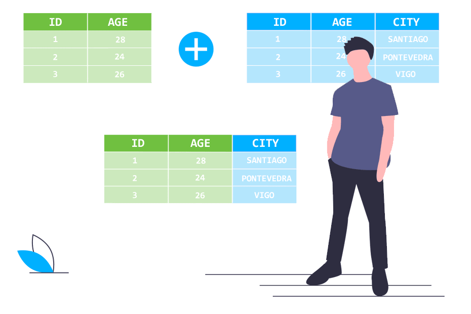
The by argument specifies the variable(s) by which you want to merge two
tables. In the picture below, it is clear that you’d want to merge both tables
using ID and AGE as by arguments. In other words, it is the common denominator.
Tipp: There are other useful ways to combine data using
the join_left() function. Have a look here.
But something isn’t right. Have a closer look….
Exactly, there are fewer observations (rows) in the new dataset compared to the students. Why is that?
Let’s take a closer look at the ID variables.
#Let's check why there are less obs in the new data

table(faculty$faculty)
##
## Business Economics Political Science Sociology
## 1 1 1 1table(faculty$faculty, useNA = "ifany")##
## Business Economics Political Science Sociology
## 1 1 1 1# now check student dataset
table(students$faculty)##
## Business Economics Political Science Sociology
## 339 225 264 162table(students$faculty, useNA = "ifany")##
## Business Economics Political Science Sociology
## 339 225 264 162
## <NA>
## 10# here is another way to look at missing values in a column
is.na(students$faculty)
sum(is.na(students$faculty))There seems to be nothing wrong with the faculty dataset. However, we
find that there are missing values in the student dataset. After further
exploration, we find that there are 10 students that have no information
on the faculty they attend. As a result, we cannot merge them with the
faculty data and the new dataset shows up with 10 observations less than
our student dataset, just as many observations as were missing in the
student dataset. The merge() function by default excludes rows that
cannot be merged. However, have a closer look at the help file for the
command. There is a way to change that setting.
# let's specify which obs we want to keep

?merge

mergeddata <- merge(students, faculty, all=TRUE)
The all=TRUE tells R to keep all rows even if they could not be
matched. When you scroll through the dataset sorted by the faculty
column, you will see that we have no faculty info (such as costs
etc.) for any students that lacks info on the faculty variable. However,
the rows are still there albeit empty in some places.
Keeping the observations with missing info may look like they’re cluttering your data but later on, you might be interested in finding out in what ways those with missing values differ from the others. For example, the info might be missing because the students dropped out before answering the survey. In that case knowing some things about the former students can still be interesting for your analysis. Long story short, there is often a reason behind missing observations, so holding on to your NA can make sense in the long run!
4.4 Appending Data
Our supervisor sent us some new student data (named students2). She
asks us to update our analysis. To do this, we need to add the rows to
our working dataset. This is called appending or in R-speak “row
binding.”
Let’s first take a look at both student datasets and check whether they have some columns in common (a key requirement for a successful bind).
# import new student data

students2 <- readxl::read_excel("data/students2.xlsx")

# check data structures

str(students)
## tibble [1,000 × 23] (S3: tbl_df/tbl/data.frame)
## $ faculty : chr [1:1000] "Business" "Business" "Business" "Business" ...
## $ course : chr [1:1000] "accounting" "accounting" "accounting" "accounting" ...
## $ age : num [1:1000] 26.3 28.8 23.9 27.4 29.3 ...
## $ cob : chr [1:1000] "Spain" "Netherlands" "Netherlands" "Spain" ...
## $ gpa_2010 : chr [1:1000] "3.1" "2.7" "1.7" "1.2" ...
## $ gpa_2011 : chr [1:1000] "2.8" "1.2" "2.5" "2.1" ...
## $ gpa_2012 : chr [1:1000] "2.8" "3.8" "3.8" "1.9" ...
## $ gpa_2013 : chr [1:1000] "2.3" "1.8" "2.9" "1.9" ...
## $ gpa_2014 : chr [1:1000] "0.5" "3" "2.4" "2.3" ...
## $ gpa_2015 : chr [1:1000] "3.9" "3" "2.4" "4.1" ...
## $ gpa_2016 : chr [1:1000] "3" "1.8" "1.6" "1" ...
## $ gpa_2017 : chr [1:1000] "1.1" "1" "3.7" "0.8" ...
## $ gpa_2018 : chr [1:1000] "2.6" "4" "2.8" "2.6" ...
## $ gpa_2019 : chr [1:1000] "3.1" "2.5" "4.1" "3.4" ...
## $ gpa_2020 : chr [1:1000] "3.9" "3" "5.7" "3.4" ...
## $ job : chr [1:1000] "no" "no" "no" "yes" ...
## $ lifesat : chr [1:1000] "68.4722360275967" "60.7386549043799" "67.2921321180378" "73.1391944810778" ...
## $ like : chr [1:1000] "3" "3" "4" "4" ...
## $ relationship: chr [1:1000] "In a relationship" "Single" "In a relationship" "Single" ...
## $ sex : chr [1:1000] "Male" "Female" "Female" "Male" ...
## $ term : chr [1:1000] "7" "4" "5" "10" ...
## $ university : chr [1:1000] "Berlin" "Berlin" "Berlin" "Berlin" ...
## $ workingclass: chr [1:1000] "yes" "yes" "no" "yes" ...str(students2)## tibble [89 × 22] (S3: tbl_df/tbl/data.frame)
## $ faculty : chr [1:89] "Business" "Business" "Business" "Business" ...
## $ course : chr [1:89] "accounting" "accounting" "accounting" "accounting" ...
## $ age : num [1:89] 27.6 24.8 25.1 21.7 29.6 ...
## $ cob : chr [1:89] "Austria" "Netherlands" "Spain" "France" ...
## $ gpa_2010 : chr [1:89] "3" "1.9" "2.4" "1.3" ...
## $ gpa_2011 : chr [1:89] "2" "3.4" "2.6" "3.8" ...
## $ gpa_2012 : chr [1:89] "2.8" "3.9" "3.6" "4.2" ...
## $ gpa_2013 : chr [1:89] "2.5" "3.4" "0.2" "2.4" ...
## $ gpa_2014 : chr [1:89] "2.8" "1.7" "2" "3.2" ...
## $ gpa_2015 : chr [1:89] "3.1" "2.2" "3.7" "2.4" ...
## $ gpa_2016 : chr [1:89] "2" "3.2" "1.3" "1.5" ...
## $ gpa_2017 : chr [1:89] "0.2" "2.2" "2.3" "0.8" ...
## $ gpa_2018 : chr [1:89] "3.9" "4.8" "2.8" "3" ...
## $ gpa_2019 : chr [1:89] "2.5" "3" "2.4" "4.2" ...
## $ gpa_2020 : chr [1:89] "5.7" "4" "4.7" "4.7" ...
## $ job : chr [1:89] "yes" "no" "no" "no" ...
## $ lifesat : chr [1:89] "37.5529004841479" "67.7055947114568" "59.3739288739801" "49.0406114404919" ...
## $ like : chr [1:89] "6" "2" "2" "4" ...
## $ sex : chr [1:89] "Female" "Male" "Male" "Male" ...
## $ term : chr [1:89] "10" "6" "4" "3" ...
## $ university : chr [1:89] "Berlin" "Berlin" "Berlin" "Berlin" ...
## $ workingclass: chr [1:89] "yes" "no" "no" "no" ...Looks like the datasets are identical in structure. So, let’s add the rows.
# now append (add rows) and save new dataset

studentsnew <- bind_rows(students, students2)
We have a new combined dataset with 1089 rows. Check out the newly added rows at the bottom of the dataset. Notice anything while browsing through?
Exactly. The new rows have missing values (“NA” = “not available”) for
the relationship variable. The bind_rows() does that
automatically when there is a column that does not exist in one of the
two datasets. This can happen often. Imagine the university stopped
asking students about their relationship status (which is highly
inappropriate anyways and somebody probably got fired over this).
Tip: Over time you may merge and append many datasets. It is highly recommend to create “id” variables to keep track of which rows came from which version. Check out the help files for each command to see how to do that (or google it).
4.5 Changing Data Structure (i.e. “Reshaping”)
Up to now, we have worked with three different datasets that we imported from excel files: students, courses, and faculty. Step by step, we have become more familiar with the data structure, what is in it and how to play with it. Why – “in the world” – would we restructure the data? Sounds complicated.
By restructuring (sometimes called “reshaping”) datasets we flip between two formats: wide and long (see Figure below). Wide means that variables are next to each other and one student is one row. Long would mean that we flip (some) columns to be underneath each other and basically put them all in one column.
In the wide format, a subject’s accumulated observations will be in
a single row, and each response is in a separate column. In the figure
below, we have three different responses from subject 1 and 2 on two
respective rows. In the long format, each row is one observation per
subject. In the figure below, we can see that each subject now occupies
three respective rows: one row per observation. Furthermore, the
structure is flipped: instead of having one id and three response
type columns, we have one id, key (response type) and val
(response) column.
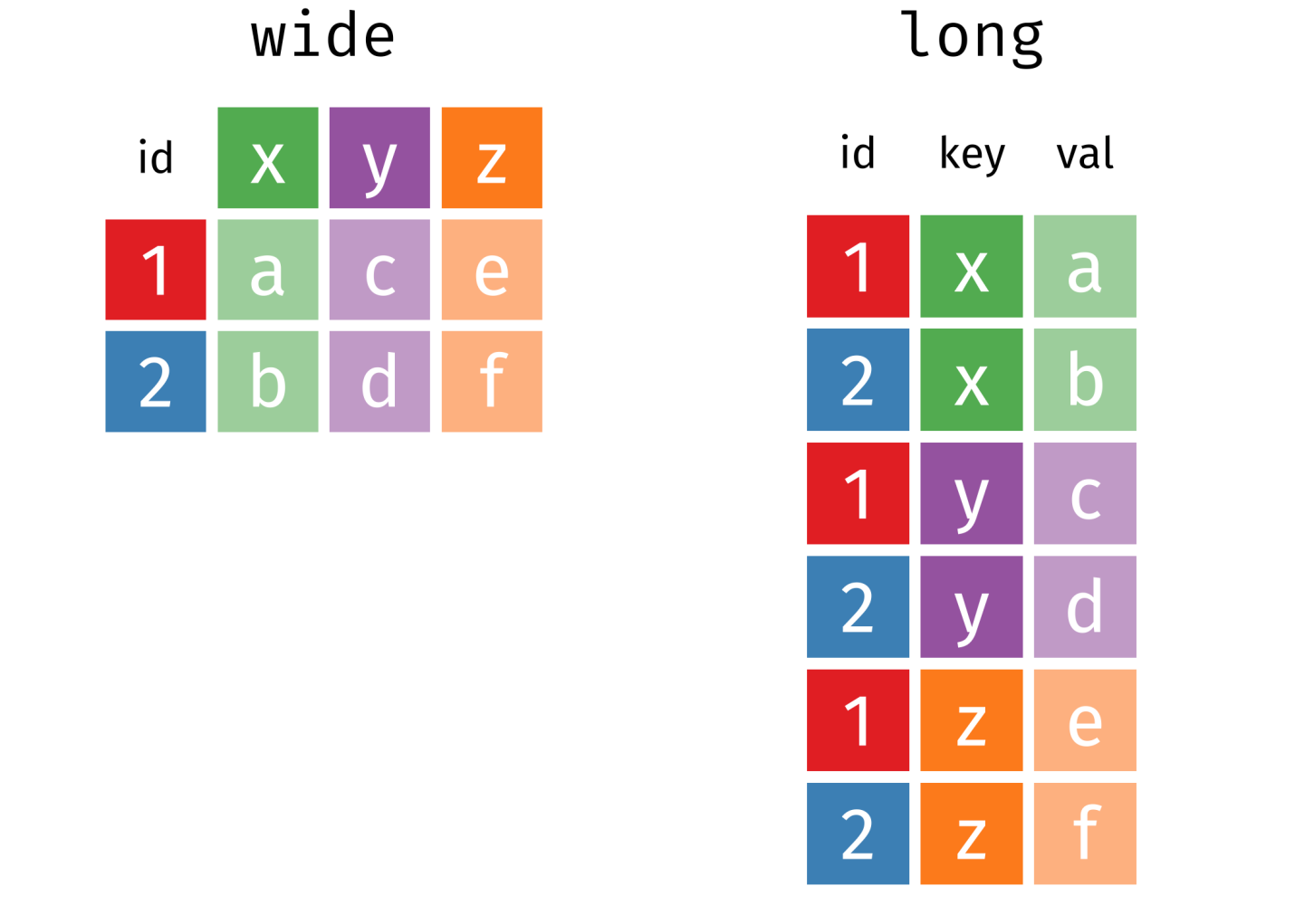
Source: https://bookdown.org/Maxine/r4ds/pivoting.html
For example, in our student data we have information on grades. We
already played around with students’ grade point average in 2010 in a
previous session. As you can see by using str() or glimpse(), we
have GPA data for 2010 all the way up to 2020, arranged in wide
format (i.e. side by side).
Why would we “reshape” the data on grades? Well, it is often easier, more convenient and quicker (especially in R) to do something to a column with many rows than to do something across multiple columns. I should say it is totally possible and sometimes advisable to keep data in wide format (as we will cover in a later session), but for simple calculations or even to do the same thing for each year of grades, the long-format has advantages. When we start producing graphics later, the involved R packages often prefer long data.
Now, let’s try to convert the grade variables to long format and then get the mean grade for each year.
# first, let's see how the function works

?pivot_longer

# convert from wide to long

students_long <- studentsnew %>% pivot_longer(cols = 5:15,
                                            names_to = "year",
                                            values_to = "grade",
                                            values_drop_na = FALSE)
cols = specifies which columns you want to turn into one, here you
select columns 5 to 15 which include the GPA data from years 2010 to
2020. Simply indicating the variables’ location spares you a lot of
tedious typing but can be risky when you’re moving around your columns a
lot. names_to = defines the name of the new variable and takes the
names of the called columns as its new values. values_to= defines
the name of the new variable that takes in the grade values.
values_drop_na = FALSE tells R not to drop/delete values that were
missing/empty.
There are different ways to specify which columns you want to restructure. Here is another way. You can tell R to convert all columns that contain a specific character/text (called “string match”):
# another way to specify the columns

students_long <- studentsnew %>% pivot_longer(cols = matches("gpa_"),
                                              names_to = "year",
                                              values_to = "grade",
                                              values_drop_na = FALSE)
Alright. Now, let’s calculate the average grade for all students by year. Luckily, we learned how to do that in the previous session. When we are done, let’s go back to a wide format.
# calculate average student grades by year

students_long <- students_long %>% group_by(year) %>%
    summarise(mean_grade = mean(grade, na.rm = TRUE))

# let's check whether this worked (It did not :-( )

students_long %>% summary(mean_grade)
## year mean_grade
## Length:11 Min. : NA
## Class :character 1st Qu.: NA
## Mode :character Median : NA
## Mean :NaN
## 3rd Qu.: NA
## Max. : NA
## NA's :11# why not?
# let's re-run previous
students_long <- studentsnew %>% pivot_longer(
cols = matches("gpa_"),
names_to = "year",
values_to = "grade",
values_drop_na = FALSE)
# let's see what kind of variable is
str(students_long)## tibble [11,979 × 14] (S3: tbl_df/tbl/data.frame)
## $ faculty : chr [1:11979] "Business" "Business" "Business" "Business" ...
## $ course : chr [1:11979] "accounting" "accounting" "accounting" "accounting" ...
## $ age : num [1:11979] 26.3 26.3 26.3 26.3 26.3 ...
## $ cob : chr [1:11979] "Spain" "Spain" "Spain" "Spain" ...
## $ job : chr [1:11979] "no" "no" "no" "no" ...
## $ lifesat : chr [1:11979] "68.4722360275967" "68.4722360275967" "68.4722360275967" "68.4722360275967" ...
## $ like : chr [1:11979] "3" "3" "3" "3" ...
## $ relationship: chr [1:11979] "In a relationship" "In a relationship" "In a relationship" "In a relationship" ...
## $ sex : chr [1:11979] "Male" "Male" "Male" "Male" ...
## $ term : chr [1:11979] "7" "7" "7" "7" ...
## $ university : chr [1:11979] "Berlin" "Berlin" "Berlin" "Berlin" ...
## $ workingclass: chr [1:11979] "yes" "yes" "yes" "yes" ...
## $ year : chr [1:11979] "gpa_2010" "gpa_2011" "gpa_2012" "gpa_2013" ...
## $ grade : chr [1:11979] "3.1" "2.8" "2.8" "2.3" ...# let's convert "grade" into a numeric variable, actually, let's do it in the same command:
students_long <- studentsnew %>% pivot_longer(cols = matches("gpa_"),
names_to = "year",
values_to = "grade",
values_drop_na = FALSE) %>%
mutate(grade = as.numeric(grade))
# it worked!
str(students_long)## tibble [11,979 × 14] (S3: tbl_df/tbl/data.frame)
## $ faculty : chr [1:11979] "Business" "Business" "Business" "Business" ...
## $ course : chr [1:11979] "accounting" "accounting" "accounting" "accounting" ...
## $ age : num [1:11979] 26.3 26.3 26.3 26.3 26.3 ...
## $ cob : chr [1:11979] "Spain" "Spain" "Spain" "Spain" ...
## $ job : chr [1:11979] "no" "no" "no" "no" ...
## $ lifesat : chr [1:11979] "68.4722360275967" "68.4722360275967" "68.4722360275967" "68.4722360275967" ...
## $ like : chr [1:11979] "3" "3" "3" "3" ...
## $ relationship: chr [1:11979] "In a relationship" "In a relationship" "In a relationship" "In a relationship" ...
## $ sex : chr [1:11979] "Male" "Male" "Male" "Male" ...
## $ term : chr [1:11979] "7" "7" "7" "7" ...
## $ university : chr [1:11979] "Berlin" "Berlin" "Berlin" "Berlin" ...
## $ workingclass: chr [1:11979] "yes" "yes" "yes" "yes" ...
## $ year : chr [1:11979] "gpa_2010" "gpa_2011" "gpa_2012" "gpa_2013" ...
## $ grade : num [1:11979] 3.1 2.8 2.8 2.3 0.5 3.9 3 1.1 2.6 3.1 ...# now, let's get the mean, still in the same command
students_long <- studentsnew %>% pivot_longer(cols = matches("gpa_"),
names_to = "year",
values_to = "grade",
values_drop_na = FALSE) %>%
mutate(grade = as.numeric(grade)) %>%
group_by(year) %>%
summarise(mean_grade = mean(grade, na.rm = TRUE))
# actually, let's the mean also by faculty and sex
students_long <- studentsnew %>% pivot_longer(cols = matches("gpa_"),
names_to = "year",
values_to = "grade",
values_drop_na = FALSE) %>%
mutate(grade = as.numeric(grade)) %>%
group_by(faculty, sex, year) %>%
summarise(mean_grade = mean(grade, na.rm = TRUE))
# now convert back to wide format
help("pivot_wider")
students_wide <- students_long %>%pivot_wider(names_from = "year",
values_from = "mean_grade")
# great, now we can merge this into the full student data
# careful - more than one id variable
full <- merge(studentsnew, students_wide, all=TRUE, by=c("faculty", "sex") )Note that we now merged the datasets based on more than one ID variable.
Together, faculty and sex uniquely identify each row in the wide
dataset. This is why we need to use them both. Also note that there are
variables in both datasets with the same name (e.g. gpa_2010). When
this happens, R automatically attaches a suffix .x or .y to
indicate from which dataset the variables originate, .x being the
first object in the merge command and .y the second.
4.6 Exercises I (based on class data)
You wake up in the middle of the night and cannot get back to sleep – the example we discussed in class was just too captivating! There is only one way to peacefully return to your slumber: you have to find out whether there is a relation between the salary of your professors and how much you and your peers enjoy your studies.
The first step is clear: You have to merge the data you have on the students with the data on the faculties like we did in class. Hint: Remember to clear your history and to load your packages and data first!
Great, now you have merged data and can proceed to explore whether students who like their course also have better paid professors. In order to do that you compute the mean salary for students who like their course and those who don’t. What do you think?
Now that you finally know, you can get back to sleep, right? Not yet. Now you are very interested in finding out more about your professors. To do so, you first load the dataset course and merge it with your previously merged data. Hint: specify a suitable ID variable!
You are interested whether the average salary of a faculty is related to the average experience of professors teaching courses at that faculty. With your newly merged dataset, you can now create a cross-tabulation of salary and professional experience – remember week two? To see which faculty provides which salary, also add a cross-tabulation for faculty and salary. For improved readability, you decide to create a categorical variable first and distinguish between three meaningful intervals of professional experience.
Finally, you want to put your fancy new pivot table skills to test. You already know how to create a pivot table with the GPA grades but this time you want to find the means by average professional experience of professors teaching the course (you can use the categorical variable from exercise 4). In order to do that, you first change the data structure to a long format based on GPA grades, group it by professional experince and year, get the mean grade and save it. Then, proceed to change the format to a wide table and merge again with the main dataframe.Explore the long and wide table you created and check which one you find more comprehensible and merge the table with the master data set. Hint: use the
pivot_longer()andpivot_wider()commands we learned in class!
Time to hit the hay!
4.7 Exercises II (based on your own data)
Revisit your individually chosen dataset. Find a suitable additional data set for you to either append or merge your data with. For example, you could append your data when finding out about a new wave of the survey you’re interested in. Surveys such as ESS or WVS usually offer the download of the complete dataset or wave by wave. Similarly, you could find a dataset with different variables you are interested in and merge it with your original data. Make sure that these variables are measured on the same unit level you’re working with, for example on country or district level.
Have a closer look at the variables in your dataset. Play around with the
pivot_longer()andpivot_wider()commands and see in what ways these can help you to get a better understanding of your data!Submit online, which data you found, why you want to merge it, how you did it (submit code) and what you learned from it. If something didn’t work, spell out what went wrong.
4.8 More helpful resources and online tutorials:
There are more ways to combine data. Check out the join function: https://dplyr.tidyverse.org/reference/join.html