5 Week 5: Producing and Exporting Tables

Up to this point, we have learned how to wrangle our data to whip it into a shape that we want for analysis. In this block of the class, we are going to learn how to conduct simple descriptive analysis, produce output, and export our work into reports. The block itself will cover four weeks in total: this week we will look at how to produce tables, the next two weeks, we will start producing figuresm and lastly, maps.

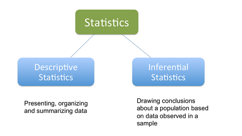
Before we jump back into R, let’s recall an important distinction in any data analysis project or statistical work: descriptive statistics and inferential statistics. Descriptive statistics is the first and important step in any analysis. It aims at “describing” your data. The description is based on averages, proportions, frequencies, and so on. The main purpose is to explore and understand the data. This is crucial to then carry out further (inferential) analysis. Descriptive analysis can already lay bare some basic relationships and patterns in the data. It can help you narrow down your research question and fine-tune your hypotheses. Importantly, it also helps you report your data in a transparent way to the reader.

Inferential statistics – ´on the other hand – is the process of drawing conclusions from your data, including methods such as hypothesis testing, multiple regression analysis, predictions, or causal designs (experimental and quasi-experimental approaches etc.). Inferential statistics (ideally) requires a very precise research question which you want to answer with the data, a theory to back up your research question, and falsifiable hypotheses and, finally, a clear research design and methodological approach. Making causal inferecens requires more advanced statistical modeling and knowledge in econometric methods.

In this course, we won’t get into inferential statistics. While it is vastly more complex and technical, that is, statistically more demanding, it (usually) consumes less time in any analysis project. Researchers, analysts, and data scientists usually spend most of their time on preparing the data and then describing it accurately.

Source: http://www.differencebetween.net/language/words-language/difference-between-descriptive-and-inferential-statistics/

Descriptive analysis uses two main instruments: Tables and Charts. In the next few weeks, we will learn how to produce effective, pretty tables and graphs and export them into various formats.

Objective of this session:

Producing and designing the right tables

R commands covered in this session:

Table()
Prop.table()
Tabyl()
Flextable()
tbl_summary()

5.1 Why Tables?

R is known for its ability to produce nice looking graphics. This – I heard many times – is one of its competitive advantages over other statistical software like Stata (side note: there are other advantages of R beyond graphics). We will handle graphics in the next two weeks, but click here and here for a sneak preview to get excited.

Naturally, I thought that producing pretty Tables in R will also be easy.

Unfortunately, it is less straight forward than I initially thought. Producing pretty tables in R might appear as an art itself. Especially in the beginning, you might feel overwhelmed. The good news is that I did the work for you and will now show you simple ways of generating tables.

5.2 Types of Tables and Terminology

So what types of tables are there?

You have surely seen many kinds of tables in reports, journals, newspapers, blogs etc. There is no commonly accepted typology or categorization of tables. Much like a matrix or a data frame, a table has rows and columns, and contains (statistical) information in each cell. However, unlike matrices or data frames, tables do not list raw data and observations, they condense information to give the reader a clear message.

Two ways of thinking about tables are:

What numbers are you interested in?
How many variables do you want to include?

Regarding 1., we have one-way tables, two-way tables, three-way and so forth. A one-way table is just a table about one variable and so on. Sometimes they are referred to as “univariate,” “bivariate” or “multivariate” (one, two or many).

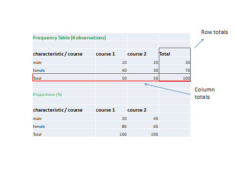
Regarding 2., broadly speaking, we have frequency tables and summary tables. Frequency tables show the number of times certain values occur in the data. In other words, we are interested in the number of rows/observations by characteristic, such as how many cats (the observation) does what kind of household category (the characteristic) have on average.

Frequency tables focus on categorical variables that have two or more categories such as sex, education, religion etc. Frequency tables struggle with continuous (metric) variables (e.g. age, income etc.). If we treated those variables like categories, there would simply be too many of them to report in one table. Imagine we would have a table reporting the number of observations for every age year. This would be too messy and not very informative. For continuous variables, we have summary tables (see below) reporting means, medians, standard deviations etc. Alternatively, you can just create new categorical variables breaking down age or income variables as we have seen in previous weeks and then use those new variables to create a frequency table.

When there is more than one variable in a frequency table, we often convert frequencies to proportions or add them alongside frequencies. Proportions show the percentage of observations per value. For example, we report there are 10 males in a course, making up 20% of all students in course 1. Two-way frequency tables are also called “contingency tables” or cross-tabs. We have used them before to check whether we recoded certain variables correctly.

Summary tables are – well – tables that summarize statistical information about data in table form. The important aspect is that we want to condense information and move away from simply reporting frequencies (although they are often also included in summary tables). Summary tables often report averages, medians, minimum values, maximum values, standard deviations etc. for multiple variables at the same time. In research papers, summary tables often combine a range of variables with different formats (categorical, continuous) and report different things at the same time. For categorical variables, summary tables usually report proportions and for continuous variables, they report averages and standard deviations.

Example of a summary table

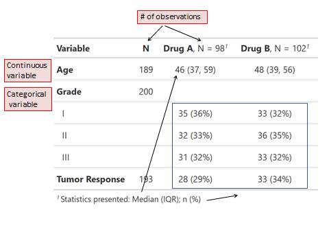
Tip: Any solid research paper or report should include summary tables to show the reader the kind of data we are dealing with to transparently describe the sample which forms the basis for later (more fancy) analyses.

5.3 Application in R

There are MANY ways to produce tables in R and there are countless packages (see e.g. here and here) to help. There is another challenge though. Normally, we do not only want to produce tables to look at them ourselves. We want to export them into something: either a Word document, Excel, a PDF, or an html report. This is where it gets a little annoying because only some packages allow you to export the data to certain formats. This aspect will be covered in a separate section (click here).

To produce tables, there are generally 3 questions you have to answer before you can even touch the keyboard:

Think about what the main information is that you would like to get out of the table:
1. Do you want to understand how a single variable is distributed?
2. Would you like to look at differences between groups?
What type of variable are you dealing with: categorical or continuous?
What do you want to see in the cells? Percentages, means, medians, modes etc.

Think about these questions first, maybe draw it up with a pen. Then start using R.

I will focus here on two broad ways to think about producing tables in R. First, think of a table just as a new data frame that you create. You use your newly acquired data management skills to produce a dataframe that includes all the information you would like to display in a table. You save it and then you use a package (in our case, flextable) to visualize the table and export it. Second, instead of “manually” creating the table yourself, use a package (in our case, gtsummary) that will produce summary stats for you using certain defaults (that you can adjust).

5.4 One-Way Frequency Tables

Ok. Let’s jump in: one-way frequency table.

###############################################################################

## APPROACH 1: Produce Table as a data frame

################

## one way frequency table (using only one variable)

# base R

tab1_1 <- as.data.frame(table(students$sex))

# apply flextable package

?flextable

flextable(tab1_1)

Var1	Freq
Female	447
Male	544

tab1_1 <- flextable(tab1_1)

tab1_1 <- set_header_labels(tab1_1, Var1 = "Respondent's Sex", Freq = "Observations")

tab1_1

Respondent's Sex	Observations
Female	447
Male	544

So, we first use the table() function to tell R to return the frequency of observations by sex variable (male vs. female respondents). The table() function requires that you tell R which data frame the variable is in using the $ sign. This is different from the tidyverse approach where we first call the data and then use the pipe operator. Thereafter, we save the table as a dataframe (not just as a list) by using the as.data.frame() function.

Tidyverse is a relatively more recent family of packages. Many R users from the first hour prefer base R approaches. The discussion is ongoing. Tidyverse – in my view – is often more intuitive and built for handling tidy data which applies to most social science studies.

Now, we have our table stored as a data frame which we called “tab1_1” and can apply the flextable() function to visualize it. The table should pop up in the viewer panel on the right-hand side. It is not pretty, but it is a start. We change the label of the columns using set_header_labels().

There are A LOT more ways to fine-tune and customize any table produced with flextable(). We will leave it in this format for now and move on to creating the same one-way frequency table using another approach.

# using "janitor package"

?tabyl

tab1_2 <- students %>% tabyl(sex)

tab1_2 <- students %>% tabyl(sex, show_na=FALSE)

flextable(tab1_2)

sex	n	percent
Female	447	0.4510595
Male	544	0.5489405

Remember the tabyl() function from the “janitor” package from last week? Again, make sure they are installed and loaded. The tabyl() function returns not only the counts (frequencies), but also the percentages: 45% of respondents in our data are female. We also tell R to exclude any missing values using show_na=FALSE. Like before, we then use the flextable() function to produce the table in the output window.

Again, there is A LOT more you can do with the tabyl() function, please explore here.

Now, off to our third approach to do the same thing. Entering the stage is the “gtsummary” package (my personal favorite).

# using gtsummary package

tab1_3 <- students %>% 
    select(sex, faculty) %>% 
    filter(faculty %in% c("Political Science", "Sociology")) %>% 
    tbl_summary()

tab1_3

Characteristic	N = 426¹
sex
Female	239 (57%)
Male	183 (43%)
Unknown	4
faculty
Political Science	264 (62%)
Sociology	162 (38%)
¹ n (%)

tab1_3 <- students %>% 
    select(sex, faculty) %>% 
    filter(faculty %in% c("Political Science", "Sociology")) %>% 
    tbl_summary(missing="no")

tab1_3

Characteristic	N = 426¹
sex
Female	239 (57%)
Male	183 (43%)
faculty
Political Science	264 (62%)
Sociology	162 (38%)
¹ n (%)

Here, the process is slightly different. You call the dataset, only keep the variable you are interested in using select(), do some filtering and then apply the tbl_summary() function. It will automatically (in most cases) detect what kind of variable you are dealing with and then provide you with either frequencies, percentages, means etc. or a combination of them.

Again, there is A LOT you can do with this package, you need to check it out here.

5.5 Two-Way Frequency Tables

So far so good. We have produced a simple one-way frequency table using three different approaches. Let us now move on to a table including two variables (two-way table). These tables are also often called cross-tabs or contingency tables. Again, we are going to use our three approaches as before: base R, janitor package and gtsummary package.

################

### cross-tab / two-way frequency table/ contingency table

## base R

tab2_1 <- table(students$cob, students$sex, useNA = c("no"))

# actually, let's convert it to proportions in percent

tab2_1 <- table(students$cob, students$sex, useNA = c("no")) %>%
                prop.table(margin = 1) %>%
                as.data.frame() %>% arrange(Var1)

# apply flextable

tab2_1 <- flextable(tab2_1)

tab2_1 <- set_header_labels(tab2_1, Var1 = "Country of origin", Var2 =
"Sex", Freq = "Obs. (%)")

tab2_1

Country of origin	Sex	Obs. (%)
Austria	Female	0.5164835
Austria	Male	0.4835165
France	Female	0.4705882
France	Male	0.5294118
Germany	Female	0.4379085
Germany	Male	0.5620915
Italy	Female	0.4452830
Italy	Male	0.5547170
Netherlands	Female	0.5000000
Netherlands	Male	0.5000000
Spain	Female	0.4402985
Spain	Male	0.5597015
UK	Female	0.4000000
UK	Male	0.6000000

Not bad, not bad. Note we used prop.table() to convert counts to proportions. Don’t forget to use the margins setting, it tells R whether you want row or column percentages. Using the %>% sign, we do it in steps: create the cross-tab, convert it to proportions, save it as data frame and lastly, sort the country of origin variable alphabetically. After that we apply flextable() to visualize the table.

Next up: janitor.

# janitor package

tab2_2 <- students %>% tabyl(cob, sex, show_na = FALSE) %>%

                            adorn_percentages("row") %>%

                            adorn_pct_formatting(digits = 2) %>%

                            adorn_ns()

tab2_2

##          cob       Female         Male
##      Austria 51.65%  (47) 48.35%  (44)
##       France 47.06%  (40) 52.94%  (45)
##      Germany 43.79%  (67) 56.21%  (86)
##        Italy 44.53% (118) 55.47% (147)
##  Netherlands 50.00%  (27) 50.00%  (27)
##        Spain 44.03% (118) 55.97% (150)
##           UK 40.00%  (30) 60.00%  (45)

Now, we made use of some of the nice customizations that tabyl() has to offer including adding percentages, formatting digits, adding observations. Does not look bad at all.

Lastly, gtsummary:

# gtsummary

tab2_3 <- students %>% select(cob,sex) %>%

                      tbl_cross(row = cob,
                                col = sex,
                                percent = "cell",
                                missing = "no",
                                label = cob ~ "Country of Origin")

tab2_3

Characteristic	sex		Total
Characteristic	Female	Male	Total
Country of Origin
Austria	47 (4.7%)	44 (4.4%)	91 (9.2%)
France	40 (4.0%)	45 (4.5%)	85 (8.6%)
Germany	67 (6.8%)	86 (8.7%)	153 (15%)
Italy	118 (12%)	147 (15%)	265 (27%)
Netherlands	27 (2.7%)	27 (2.7%)	54 (5.4%)
Spain	118 (12%)	150 (15%)	268 (27%)
UK	30 (3.0%)	45 (4.5%)	75 (7.6%)
Total	447 (45%)	544 (55%)	991 (100%)

Note that we used tbl_cross() – a special function just for cross-tabs. We also used some more details such as adding percentages, excluding missing information and changing the label of a variable.

5.6 Three-Way Frequency Tables

Let’s try a three-way table showing information for a combination of three variables, in our case, for country of birth, sex and relationship status. The approach we are going to take is by manually calculating the table contents and saving it a long format. We will do that using some of our recently acquired data management skills, so this will be useful repetition.

# Three-way table

tab3 <- students %>% select(cob, sex, relationship) %>%

                    group_by(cob, sex, relationship) %>%
                    
                    summarise(n = n()) %>%
                    
                    group_by(cob, sex) %>%
                    
                    mutate(percent = n/sum(n)*100) %>%
                    
                    filter(!is.na(cob)) %>%

                    pivot_wider(names_from = "sex", values_from = c("n", "percent"))

flextable(tab3)

cob	relationship	n_Female	n_Male	percent_Female	percent_Male
Austria	In a relationship	13	11	27.65957	25.00000
Austria	Single	34	33	72.34043	75.00000
France	In a relationship	10	16	25.00000	35.55556
France	Single	30	29	75.00000	64.44444
Germany	In a relationship	16	35	23.88060	40.69767
Germany	Single	51	51	76.11940	59.30233
Italy	In a relationship	28	44	23.72881	29.93197
Italy	Single	90	103	76.27119	70.06803
Netherlands	In a relationship	10	9	37.03704	33.33333
Netherlands	Single	17	18	62.96296	66.66667
Spain	In a relationship	36	44	30.50847	29.33333
Spain	Single	82	106	69.49153	70.66667
UK	In a relationship	10	13	33.33333	28.88889
UK	Single	20	32	66.66667	71.11111

If you read out the code above, it would sound like this:

Save a new object called tab3; in it, put the students dataframe, only keep cob, sex and relationship as columns in the dataframe. Group the data by every combination of cob, sex, and relationship and then count how many observations there are for each one of those combinations (summarise()). Afterwards, group by cob and sex and subsequently generate a new variable that contains the percentage distribution of relationship statuses. Exclude any row that have no info on cob (!is.na()) – the is.na() function is helpful. It refers to all observations that are “not available” (i.e. missing). The ! operator applies the opposite, so “Not missing.” Lastly, convert the data frame into a wide format, generating columns for males and females. VoilC !

Now, apply flextable() and we have a three-way table.

Tip: Think hard about whether you really need a three-way table. They can get quite complex for the reader. It might be easier to create a graph which communicates the main message more clearly than a three-way table.

5.7 Summary Tables

Alright. We have now entered the end game. The last table we will learn to produce is a full summary table. By that I mean that we will present a summary of multiple variables irrespective of their variable type (categorical, continuous etc.). Summary tables are common in academic papers because they describe the sample that is used for more advanced analysis. Usually, a summary table includes all variables that are used, for example, in statistical modelling.

Some people create separate tables for categorical variables (reporting percentages) and continuous variables (reporting means, medians, standard deviations, min, max etc.). These are quicker to produce, and since the statistics that are reported differ quite a bit, you do not have to worry about harmonizing the format and layout.

Another trick is to recode categorical variables into a set of so-called “dummy” (or binary) variables. For example, you have a variable called religion: 1 – Christian 2 – Muslim 3- Jewish – 4 Other. This is a classic categorical variable. If you divide it up into dummies, the variable will split into 4 separate variables each indicating yes or no. Christian: TRUE/FALSE (0/1), Muslim: TRUE/FALSE (0/1) and so on. When you do this for all categorical variables, you can run create the mean for all variables. The mean for a binary variable (0-1) can easily be converted to percentages by multiplying by 100.

Anyways…apologies for the long detour. We will be doing neither of the two above approaches. Instead, we will apply the gtsummary package. It is fairly easy and – at the same time – elegant.

#### SUMMARY Table

tab4_1 <- students %>% 
    select(cob, sex, relationship, age, term, lifesat, job) %>%
    tbl_summary()

Characteristic	N = 1,000
cob
Austria	91 (9.2%)
France	85 (8.6%)
Germany	153 (15%)
Italy	265 (27%)
Netherlands	54 (5.4%)
Spain	268 (27%)
UK	75 (7.6%)
Unknown	9
sex
Female	447 (45%)
Male	544 (55%)
Unknown	9
relationship
In a relationship	295 (30%)
Single	696 (70%)
Unknown	9
age	25.9 (23.7, 28.0)
Unknown	9
term
0	69 (7.0%)
1	57 (5.8%)
10	64 (6.5%)
11	66 (6.7%)
12	69 (7.0%)
13	60 (6.1%)
14	62 (6.3%)
2	60 (6.1%)
3	67 (6.8%)
4	66 (6.7%)
5	70 (7.1%)
6	61 (6.2%)
7	71 (7.2%)
8	75 (7.6%)
9	74 (7.5%)
Unknown	9
lifesat
0	1 (0.1%)
0.45737256977358	1 (0.1%)
10.1772689702957	1 (0.1%)
10.7664921543563	1 (0.1%)
100	1 (0.1%)
11.6944049446601	1 (0.1%)
13.4706560828935	1 (0.1%)
14.5707574169521	1 (0.1%)
15.4820684475481	1 (0.1%)
15.5810206873513	1 (0.1%)
17.2866231806492	1 (0.1%)
17.6087433252336	1 (0.1%)
17.9793495176851	1 (0.1%)
18.1156054498785	1 (0.1%)
18.3724102438826	1 (0.1%)
18.567949960643	1 (0.1%)
18.9376945184199	1 (0.1%)
18.9857394583137	1 (0.1%)
19.3995543852231	1 (0.1%)
2.69900005888443	1 (0.1%)
20.6227359388643	1 (0.1%)
21.1214757016822	1 (0.1%)
21.9703912522502	1 (0.1%)
22.0749804384493	1 (0.1%)
22.6116046722593	1 (0.1%)
22.773853782585	1 (0.1%)
23.0976026518452	1 (0.1%)
23.4685350503946	1 (0.1%)
23.5123466847752	1 (0.1%)
24.8657878376206	1 (0.1%)
24.8844840378305	1 (0.1%)
25.2794616959529	1 (0.1%)
25.8253397770735	1 (0.1%)
25.8726627790811	1 (0.1%)
26.6238085186153	1 (0.1%)
27.1747837193627	1 (0.1%)
27.5760931224349	1 (0.1%)
27.713707658821	1 (0.1%)
27.7375678511294	1 (0.1%)
27.7516547183653	1 (0.1%)
27.9015348742358	1 (0.1%)
28.2891060125721	1 (0.1%)
28.4551472491259	1 (0.1%)
28.4798025148595	1 (0.1%)
28.5979221759001	1 (0.1%)
28.6436796557387	1 (0.1%)
28.9799267515966	1 (0.1%)
29.1509858212042	1 (0.1%)
29.2042479851419	1 (0.1%)
29.2572407993707	1 (0.1%)
29.3122950503655	1 (0.1%)
29.3728834305609	1 (0.1%)
29.8533706933198	1 (0.1%)
30.1156965728573	1 (0.1%)
30.1359106383616	1 (0.1%)
30.3150650548278	1 (0.1%)
30.7219599417264	1 (0.1%)
30.7414719272093	1 (0.1%)
30.821240879999	1 (0.1%)
30.8345235755115	1 (0.1%)
31.3464231563294	1 (0.1%)
31.9636513167819	1 (0.1%)
31.9790634894965	1 (0.1%)
32.1822774034271	1 (0.1%)
32.2904142490675	1 (0.1%)
32.3117693155517	1 (0.1%)
32.494283665968	1 (0.1%)
32.6918739806539	1 (0.1%)
32.7501546477674	1 (0.1%)
32.828047687616	1 (0.1%)
33.1177864710646	1 (0.1%)
33.1588329262009	1 (0.1%)
33.3050680592648	1 (0.1%)
33.4028064293051	1 (0.1%)
33.5000060864196	1 (0.1%)
33.5470268394014	1 (0.1%)
33.6378970674729	1 (0.1%)
33.764615408307	1 (0.1%)
34.031362004637	1 (0.1%)
34.083736013337	1 (0.1%)
34.1125916625418	1 (0.1%)
34.1941117922674	1 (0.1%)
34.2199791004803	1 (0.1%)
34.323821220121	1 (0.1%)
34.4014345222505	1 (0.1%)
34.4110411763486	1 (0.1%)
34.449825947388	1 (0.1%)
34.5027903639557	1 (0.1%)
34.5930844880203	1 (0.1%)
34.6468895886108	1 (0.1%)
34.812759657136	1 (0.1%)
34.9070730087366	1 (0.1%)
34.9548877271729	1 (0.1%)
35.0317097927783	1 (0.1%)
35.0603736014297	1 (0.1%)
35.0662908338391	1 (0.1%)
35.1312513244583	1 (0.1%)
35.1952972464747	1 (0.1%)
35.2273402476762	1 (0.1%)
35.2850492214444	1 (0.1%)
35.3139720657457	1 (0.1%)
35.3553502881286	1 (0.1%)
35.3862621356601	1 (0.1%)
35.4645224792207	1 (0.1%)
35.6271218763781	1 (0.1%)
35.6441566638026	1 (0.1%)
35.8255613381041	1 (0.1%)
35.8921617139823	1 (0.1%)
35.893817131199	1 (0.1%)
35.9438376630607	1 (0.1%)
36.1618346035622	1 (0.1%)
36.1726195757006	1 (0.1%)
36.1993857901107	1 (0.1%)
36.3818203719286	1 (0.1%)
36.6128051943683	1 (0.1%)
36.6219330646692	1 (0.1%)
36.7329721480909	1 (0.1%)
36.8463981737829	1 (0.1%)
36.9717925318144	1 (0.1%)
37.0956197062207	1 (0.1%)
37.2113077228484	1 (0.1%)
37.471119425269	1 (0.1%)
37.5529004841479	1 (0.1%)
37.5893499373533	1 (0.1%)
37.6125611455419	1 (0.1%)
37.6312492172009	1 (0.1%)
37.7361625275507	1 (0.1%)
37.7453851320127	1 (0.1%)
38.0036137925878	1 (0.1%)
38.1565384673941	1 (0.1%)
38.1990868197832	1 (0.1%)
38.234940361373	1 (0.1%)
38.2382025088838	1 (0.1%)
38.3118631638634	1 (0.1%)
38.4168492448223	1 (0.1%)
38.4962130631582	1 (0.1%)
38.6473768282327	1 (0.1%)
38.819812404157	1 (0.1%)
38.9170870269999	1 (0.1%)
39.1224840929615	1 (0.1%)
39.2781336450114	1 (0.1%)
39.2896121006286	1 (0.1%)
39.3779905493502	1 (0.1%)
39.5488912568947	1 (0.1%)
39.5494712841438	1 (0.1%)
39.6103117455723	1 (0.1%)
39.7139988412579	1 (0.1%)
39.8423460961231	1 (0.1%)
39.9577794403425	1 (0.1%)
40.0209440186605	1 (0.1%)
40.4055723159926	1 (0.1%)
40.4941814886201	1 (0.1%)
40.5058965001633	1 (0.1%)
40.6460776804788	1 (0.1%)
40.7622088297377	1 (0.1%)
40.843590317379	1 (0.1%)
40.9374156383302	1 (0.1%)
41.1115780026849	1 (0.1%)
41.2801328895737	1 (0.1%)
41.320832552613	1 (0.1%)
41.3394995993083	1 (0.1%)
41.4147270622808	1 (0.1%)
41.6858657127112	1 (0.1%)
41.8310804172791	1 (0.1%)
41.8592689392941	1 (0.1%)
41.9819497127695	1 (0.1%)
42.0714607682833	1 (0.1%)
42.1560787250141	1 (0.1%)
42.1696700825123	1 (0.1%)
42.260223144515	1 (0.1%)
42.2707018473124	1 (0.1%)
42.2750810335129	1 (0.1%)
42.2891505492271	1 (0.1%)
42.4344379549119	1 (0.1%)
42.4784377198514	1 (0.1%)
42.5465795188766	1 (0.1%)
42.8038638557009	1 (0.1%)
43.1364065045377	1 (0.1%)
43.1925758962142	1 (0.1%)
43.2336307483222	1 (0.1%)
43.4280895829189	1 (0.1%)
43.4613162162932	1 (0.1%)
43.466644086287	1 (0.1%)
43.4990341961584	1 (0.1%)
43.7544142071821	1 (0.1%)
43.8191069586458	1 (0.1%)
43.8521975367342	1 (0.1%)
43.9198279709853	1 (0.1%)
43.9955337283186	1 (0.1%)
44.0597191277837	1 (0.1%)
44.2567133956319	1 (0.1%)
44.3495606371963	1 (0.1%)
44.3933981169638	1 (0.1%)
44.4108722764608	1 (0.1%)
44.517075305689	1 (0.1%)
44.5739455454796	1 (0.1%)
44.6817224242127	1 (0.1%)
45.0554449486089	1 (0.1%)
45.0824179132679	1 (0.1%)
45.2210440422524	1 (0.1%)
45.2721894871145	1 (0.1%)
45.3233063417645	1 (0.1%)
45.3771284828732	1 (0.1%)
45.380331382467	1 (0.1%)
45.4488532762662	1 (0.1%)
45.48606175981	1 (0.1%)
45.5554319711532	1 (0.1%)
45.5817489031739	1 (0.1%)
45.6162837889357	1 (0.1%)
45.6428364385974	1 (0.1%)
45.6479860744964	1 (0.1%)
45.6947404120311	1 (0.1%)
45.7078441319471	1 (0.1%)
45.7302717071732	1 (0.1%)
45.7914420112966	1 (0.1%)
45.8327060793355	1 (0.1%)
45.8634026871598	1 (0.1%)
45.8647490799655	1 (0.1%)
45.9214695844258	1 (0.1%)
45.9369757871	1 (0.1%)
45.9967602913201	1 (0.1%)
46.0052974067049	1 (0.1%)
46.1051734117191	1 (0.1%)
46.179942122366	1 (0.1%)
46.2159179268147	1 (0.1%)
46.4063107943336	1 (0.1%)
46.4488725111043	1 (0.1%)
46.52002793419	1 (0.1%)
46.530425403641	1 (0.1%)
46.575520126841	1 (0.1%)
46.6072260940315	1 (0.1%)
46.6281054977917	1 (0.1%)
46.6343328627899	1 (0.1%)
46.6890160113622	1 (0.1%)
46.6969768535315	1 (0.1%)
46.7604025995515	1 (0.1%)
46.777210498315	1 (0.1%)
46.8147326225005	1 (0.1%)
46.9111915831809	1 (0.1%)
46.9121373960911	1 (0.1%)
46.9221416794523	1 (0.1%)
46.943803828629	1 (0.1%)
47.0218567308489	1 (0.1%)
47.1275555937762	1 (0.1%)
47.1415793582149	1 (0.1%)
47.1560070056092	1 (0.1%)
47.1746083707061	1 (0.1%)
47.2129192908701	1 (0.1%)
47.2450668663347	1 (0.1%)
47.3061497417086	1 (0.1%)
47.3655863027285	1 (0.1%)
47.3991519790613	1 (0.1%)
47.4133154661436	1 (0.1%)
47.423980274673	1 (0.1%)
47.439768556172	1 (0.1%)
47.4646389511972	1 (0.1%)
47.5039710519267	1 (0.1%)
47.5698819822193	1 (0.1%)
47.579898622523	1 (0.1%)
47.614618386054	1 (0.1%)
47.7438319660412	1 (0.1%)
47.8857170386222	1 (0.1%)
47.9869065908174	1 (0.1%)
47.9923249126504	1 (0.1%)
48.0357730008347	1 (0.1%)
48.0848793929655	1 (0.1%)
48.1477237474873	1 (0.1%)
48.2261555858052	1 (0.1%)
48.2955739833277	1 (0.1%)
48.3016772967098	1 (0.1%)
48.3128615070933	1 (0.1%)
48.4120395189983	1 (0.1%)
48.4437257827297	1 (0.1%)
48.4457135666961	1 (0.1%)
48.4785409060363	1 (0.1%)
48.5157697910372	1 (0.1%)
48.545198262508	1 (0.1%)
48.6523878049085	1 (0.1%)
48.656358232708	1 (0.1%)
48.6900357763617	1 (0.1%)
48.6994418652197	1 (0.1%)
48.7498144496244	1 (0.1%)
48.7988006091344	1 (0.1%)
48.8646793685281	1 (0.1%)
48.8732400170919	1 (0.1%)
48.8837388080093	1 (0.1%)
49.0406114404919	1 (0.1%)
49.0796026009137	1 (0.1%)
49.0992590631285	1 (0.1%)
49.1810078932101	1 (0.1%)
49.212687740506	1 (0.1%)
49.2593795174238	1 (0.1%)
49.5269905585214	1 (0.1%)
49.5873786608714	1 (0.1%)
49.6018254745951	1 (0.1%)
49.6226069749221	1 (0.1%)
49.6320810073961	1 (0.1%)
49.6928995513887	1 (0.1%)
49.7411707955502	1 (0.1%)
49.7746621686557	1 (0.1%)
49.8624670145065	1 (0.1%)
49.8917727974103	1 (0.1%)
49.9343677005329	1 (0.1%)
50.0044230809663	1 (0.1%)
50.1004024413061	1 (0.1%)
50.3787247305083	1 (0.1%)
50.4192456344854	1 (0.1%)
50.4877443368157	1 (0.1%)
50.5497932995187	1 (0.1%)
50.563489234732	1 (0.1%)
50.6152307084525	1 (0.1%)
50.621926418489	1 (0.1%)
50.6722486256882	1 (0.1%)
50.7685788418511	1 (0.1%)
50.7770630472402	1 (0.1%)
50.8712260626278	1 (0.1%)
50.8823056988445	1 (0.1%)
50.9067626580991	1 (0.1%)
50.911523627437	1 (0.1%)
50.926964347229	1 (0.1%)
50.9529118587314	1 (0.1%)
50.9740080233511	1 (0.1%)
51.0026018978105	1 (0.1%)
51.0092612478704	1 (0.1%)
51.0556167566072	1 (0.1%)
51.0580542191253	1 (0.1%)
51.0716640462018	1 (0.1%)
51.1028484547497	1 (0.1%)
51.2054281747299	1 (0.1%)
51.2398127286987	1 (0.1%)
51.2756152416379	1 (0.1%)
51.2797233179465	1 (0.1%)
51.2860049616198	1 (0.1%)
51.3585465968472	1 (0.1%)
51.4107195939913	1 (0.1%)
51.4238969491782	1 (0.1%)
51.4600144392702	1 (0.1%)
51.5223670275746	1 (0.1%)
51.572241434378	1 (0.1%)
51.5783649889135	1 (0.1%)
51.6933874511186	1 (0.1%)
51.708993274882	1 (0.1%)
51.7126978957526	1 (0.1%)
51.7202145469544	1 (0.1%)
51.7727624169722	1 (0.1%)
51.8273555914468	1 (0.1%)
51.8747761319067	1 (0.1%)
51.9533951389037	1 (0.1%)
51.961348935387	1 (0.1%)
51.9803315763116	1 (0.1%)
52.0323015501357	1 (0.1%)
52.032497242053	1 (0.1%)
52.0671660470746	1 (0.1%)
52.1323756590309	1 (0.1%)
52.3509402599681	1 (0.1%)
52.3568858318556	1 (0.1%)
52.4006128797986	1 (0.1%)
52.4542002688105	1 (0.1%)
52.4591064899991	1 (0.1%)
52.5680601129846	1 (0.1%)
52.5685690660695	1 (0.1%)
52.614760290092	1 (0.1%)
52.6264224478868	1 (0.1%)
52.6561155785406	1 (0.1%)
52.6762233786903	1 (0.1%)
52.6839126579608	1 (0.1%)
52.6991633627189	1 (0.1%)
52.7529996396389	1 (0.1%)
52.7789994911054	1 (0.1%)
52.7929295676129	1 (0.1%)
52.8374050831156	1 (0.1%)
52.91690464414	1 (0.1%)
53.0055438743309	1 (0.1%)
53.0605525820135	1 (0.1%)
53.0975117601682	1 (0.1%)
53.2260952145181	1 (0.1%)
53.2605439691821	1 (0.1%)
53.2624641918695	1 (0.1%)
53.2685185887926	1 (0.1%)
53.2998819732859	1 (0.1%)
53.3318615807103	1 (0.1%)
53.375384933806	1 (0.1%)
53.4004110035826	1 (0.1%)
53.5233289348475	1 (0.1%)
53.5843763525849	1 (0.1%)
53.633575262961	1 (0.1%)
53.7820232950468	1 (0.1%)
53.8504454176038	1 (0.1%)
53.8583720524614	1 (0.1%)
53.9316740466018	1 (0.1%)
53.9634911857525	1 (0.1%)
53.9886006228042	1 (0.1%)
54.0576406022764	1 (0.1%)
54.0623263291074	1 (0.1%)
54.1365806644279	1 (0.1%)
54.1511570538146	1 (0.1%)
54.1733864465202	1 (0.1%)
54.1798602154755	1 (0.1%)
54.1958820266782	1 (0.1%)
54.2057115150397	1 (0.1%)
54.2140383606153	1 (0.1%)
54.2286757429389	1 (0.1%)
54.3088943000751	1 (0.1%)
54.4436682843346	1 (0.1%)
54.4524283750509	1 (0.1%)
54.4940231691635	1 (0.1%)
54.5734856517324	1 (0.1%)
54.5970057517337	1 (0.1%)
54.6346072241927	1 (0.1%)
54.6768194712138	1 (0.1%)
54.7908398445326	1 (0.1%)
54.8016905691657	1 (0.1%)
54.811176534094	1 (0.1%)
54.8650679112415	1 (0.1%)
54.9012902850452	1 (0.1%)
54.9021291450848	1 (0.1%)
54.9039358820183	1 (0.1%)
54.9778499129789	1 (0.1%)
55.0085745069251	1 (0.1%)
55.1186630242204	1 (0.1%)
55.1778130133868	1 (0.1%)
55.1817485422905	1 (0.1%)
55.1975300055561	1 (0.1%)
55.2343433844774	1 (0.1%)
55.2408263078844	1 (0.1%)
55.2940515962946	1 (0.1%)
55.3003535309783	1 (0.1%)
55.4045179459406	1 (0.1%)
55.5212153608845	1 (0.1%)
55.7658603771912	1 (0.1%)
55.8332211058468	1 (0.1%)
55.8526129815954	1 (0.1%)
55.9506009251173	1 (0.1%)
55.9543976619673	1 (0.1%)
56.0724275150502	1 (0.1%)
56.0744260310992	1 (0.1%)
56.1077453360638	1 (0.1%)
56.1102043320017	1 (0.1%)
56.1196214912576	1 (0.1%)
56.1280887945436	1 (0.1%)
56.1291188260406	1 (0.1%)
56.1555922619776	1 (0.1%)
56.2203286635155	1 (0.1%)
56.2580299901415	1 (0.1%)
56.2999513383797	1 (0.1%)
56.4169686269331	1 (0.1%)
56.4487080906771	1 (0.1%)
56.4708228123194	1 (0.1%)
56.4958518847945	1 (0.1%)
56.5228767296023	1 (0.1%)
56.5392970891723	1 (0.1%)
56.5898443048144	1 (0.1%)
56.6274543721398	1 (0.1%)
56.6579314246458	1 (0.1%)
56.6879384294575	1 (0.1%)
56.7863229679663	1 (0.1%)
56.8410504171307	1 (0.1%)
56.8581506009311	1 (0.1%)
56.9100951365115	1 (0.1%)
57.1740535639203	1 (0.1%)
57.2320080979754	1 (0.1%)
57.2638319909575	1 (0.1%)
57.2805837860595	1 (0.1%)
57.3296113574152	1 (0.1%)
57.3634373694223	1 (0.1%)
57.373906249777	1 (0.1%)
57.3831782315293	1 (0.1%)
57.4581329999836	1 (0.1%)
57.4835302023715	1 (0.1%)
57.5056773777073	1 (0.1%)
57.601019740241	1 (0.1%)
57.8443788083101	1 (0.1%)
57.8822895822692	1 (0.1%)
57.8877453226317	1 (0.1%)
57.909059461553	1 (0.1%)
58.1236696110713	1 (0.1%)
58.125833263771	1 (0.1%)
58.1325583905772	1 (0.1%)
58.1667127686433	1 (0.1%)
58.1802413095173	1 (0.1%)
58.1987398250567	1 (0.1%)
58.2179302027876	1 (0.1%)
58.2192085502738	1 (0.1%)
58.2675867678329	1 (0.1%)
58.3099048284602	1 (0.1%)
58.3581213094002	1 (0.1%)
58.3710699326806	1 (0.1%)
58.4335184823223	1 (0.1%)
58.446386556742	1 (0.1%)
58.4967882618003	1 (0.1%)
58.506705435258	1 (0.1%)
58.5120616545272	1 (0.1%)
58.5490404975145	1 (0.1%)
58.5727370460607	1 (0.1%)
58.5785275509716	1 (0.1%)
58.6009022994813	1 (0.1%)
58.6213575810484	1 (0.1%)
58.6573980127333	1 (0.1%)
58.6690845256988	1 (0.1%)
58.8317529467956	1 (0.1%)
58.8377743593965	1 (0.1%)
58.8689745561489	1 (0.1%)
58.8751068816297	1 (0.1%)
58.9800567063813	1 (0.1%)
59.0367763520852	1 (0.1%)
59.0564826031682	1 (0.1%)
59.0609002562039	1 (0.1%)
59.1316814133124	1 (0.1%)
59.1951408046069	1 (0.1%)
59.198319805236	1 (0.1%)
59.2776190787508	1 (0.1%)
59.3739288739801	1 (0.1%)
59.3785095831942	1 (0.1%)
59.4283156222694	1 (0.1%)
59.4581267548125	1 (0.1%)
59.4762674227016	1 (0.1%)
59.4786443989519	1 (0.1%)
59.5187867209421	1 (0.1%)
59.5552779678312	1 (0.1%)
59.5931918715955	1 (0.1%)
59.5959747006596	1 (0.1%)
59.6164490311472	1 (0.1%)
59.6380870106413	1 (0.1%)
59.6492741012975	1 (0.1%)
59.7026284396004	1 (0.1%)
59.709544879239	1 (0.1%)
59.9027242180549	1 (0.1%)
59.9201634765974	1 (0.1%)
59.9357211793107	1 (0.1%)
59.9378546412141	1 (0.1%)
59.9544160356755	1 (0.1%)
59.9685511723383	1 (0.1%)
60.0070139835876	1 (0.1%)
60.0079208916958	1 (0.1%)
60.0283290970283	1 (0.1%)
60.0613493480594	1 (0.1%)
60.0929406775432	1 (0.1%)
60.1017774804349	1 (0.1%)
60.2624815102779	1 (0.1%)
60.3091920151294	1 (0.1%)
60.3222545489635	1 (0.1%)
60.3343733937268	1 (0.1%)
60.5045176346209	1 (0.1%)
60.5050372848552	1 (0.1%)
60.5167269832529	1 (0.1%)
60.5856193503402	1 (0.1%)
60.5895046710715	1 (0.1%)
60.6990925112276	1 (0.1%)
60.7009775970221	1 (0.1%)
60.7012093959081	1 (0.1%)
60.7068448257743	1 (0.1%)
60.7386549043799	1 (0.1%)
60.7519672707165	1 (0.1%)
60.7545973759783	1 (0.1%)
60.7941912098927	1 (0.1%)
60.8292586293271	1 (0.1%)
60.8409395477149	1 (0.1%)
60.8701783158278	1 (0.1%)
60.9225882941788	1 (0.1%)
60.9290374005205	1 (0.1%)
60.9429160013578	1 (0.1%)
60.9614966798592	1 (0.1%)
60.973033075194	1 (0.1%)
61.078326320554	1 (0.1%)
61.0915867334923	1 (0.1%)
61.115397885497	1 (0.1%)
61.1169851169854	1 (0.1%)
61.1737369652881	1 (0.1%)
61.3506946117744	1 (0.1%)
61.4653225262189	1 (0.1%)
61.4862355026893	1 (0.1%)
61.5667264529059	1 (0.1%)
61.6577423010377	1 (0.1%)
61.6791489022296	1 (0.1%)
61.6990423419784	1 (0.1%)
61.7345654840901	1 (0.1%)
61.753615901867	1 (0.1%)
61.8391698212221	1 (0.1%)
61.8692105393297	1 (0.1%)
61.9142327826884	1 (0.1%)
61.9408959625775	1 (0.1%)
62.0307236862006	1 (0.1%)
62.0327344537313	1 (0.1%)
62.0719665102692	1 (0.1%)
62.1031532172894	1 (0.1%)
62.1691873145667	1 (0.1%)
62.1963987188102	1 (0.1%)
62.2805326810222	1 (0.1%)
62.3104088846814	1 (0.1%)
62.3169294789505	1 (0.1%)
62.3438697376796	1 (0.1%)
62.4073299835186	1 (0.1%)
62.4210619289664	1 (0.1%)
62.4505709084755	1 (0.1%)
62.5025297073763	1 (0.1%)
62.7243512774508	1 (0.1%)
62.7370309149722	1 (0.1%)
62.7846450408817	1 (0.1%)
62.8372532501836	1 (0.1%)
62.8436827617527	1 (0.1%)
62.8782287220068	1 (0.1%)
62.9087119839042	1 (0.1%)
62.9110367504478	1 (0.1%)
62.94869233016	1 (0.1%)
62.9866482482273	1 (0.1%)
62.9981807908279	1 (0.1%)
63.0251570516857	1 (0.1%)
63.2018393172069	1 (0.1%)
63.233678640069	1 (0.1%)
63.2689910700214	1 (0.1%)
63.316399571602	1 (0.1%)
63.3182591054446	1 (0.1%)
63.3440370351027	1 (0.1%)
63.4095537254159	1 (0.1%)
63.4292297764367	1 (0.1%)
63.4562409431074	1 (0.1%)
63.4757614073261	1 (0.1%)
63.5147233616682	1 (0.1%)
63.5387286433099	1 (0.1%)
63.5507935810719	1 (0.1%)
63.589342558872	1 (0.1%)
63.6033937646625	1 (0.1%)
63.6170109351586	1 (0.1%)
63.6442993068965	1 (0.1%)
63.709389556104	1 (0.1%)
63.7286351601193	1 (0.1%)
63.771592863813	1 (0.1%)
63.8440961521691	1 (0.1%)
63.8734254774071	1 (0.1%)
63.900152718628	1 (0.1%)
63.975165613289	1 (0.1%)
63.99036546092	1 (0.1%)
64.0645620854423	1 (0.1%)
64.1609424160786	1 (0.1%)
64.163941747842	1 (0.1%)
64.2579986931741	1 (0.1%)
64.3722329036194	1 (0.1%)
64.3773409150661	1 (0.1%)
64.4590837519135	1 (0.1%)
64.49231786731	1 (0.1%)
64.5142994001936	1 (0.1%)
64.5695932739959	1 (0.1%)
64.5776281535838	1 (0.1%)
64.7484018898	1 (0.1%)
64.7880575921934	1 (0.1%)
64.8129892554265	1 (0.1%)
64.8447621333077	1 (0.1%)
64.8642467102503	1 (0.1%)
64.9111146159861	1 (0.1%)
64.9772997504887	1 (0.1%)
65.1656101209698	1 (0.1%)
65.1879927400937	1 (0.1%)
65.2452396058935	1 (0.1%)
65.3046653793866	1 (0.1%)
65.310499266934	1 (0.1%)
65.3937922846809	1 (0.1%)
65.4480208633053	1 (0.1%)
65.450481126591	1 (0.1%)
65.4815314037498	1 (0.1%)
65.5521573874841	1 (0.1%)
65.5869783575206	1 (0.1%)
65.6789148917245	1 (0.1%)
65.6837597523699	1 (0.1%)
65.6935776780863	1 (0.1%)
65.7190836211296	1 (0.1%)
65.7266789062011	1 (0.1%)
65.7825163063419	1 (0.1%)
65.7968855332173	1 (0.1%)
65.914140358838	1 (0.1%)
65.9249426828103	1 (0.1%)
65.9585842250699	1 (0.1%)
65.9693259857039	1 (0.1%)
65.9918231190594	1 (0.1%)
66.0507964351298	1 (0.1%)
66.0606957808595	1 (0.1%)
66.1709533614314	1 (0.1%)
66.2191143228235	1 (0.1%)
66.3196612758953	1 (0.1%)
66.3313679705396	1 (0.1%)
66.4202049103437	1 (0.1%)
66.4205925118002	1 (0.1%)
66.441888261832	1 (0.1%)
66.4917438866905	1 (0.1%)
66.8062948675913	1 (0.1%)
66.8408466537074	1 (0.1%)
66.9673204187453	1 (0.1%)
67.0832601759517	1 (0.1%)
67.0884003693873	1 (0.1%)
67.0941533695824	1 (0.1%)
67.1630396739757	1 (0.1%)
67.2921321180378	1 (0.1%)
67.3057019818387	1 (0.1%)
67.3073115206282	1 (0.1%)
67.4336646437078	1 (0.1%)
67.4356710181492	1 (0.1%)
67.4956733246418	1 (0.1%)
67.5015394545924	1 (0.1%)
67.5360248408889	1 (0.1%)
67.5763739590983	1 (0.1%)
67.6439045094589	1 (0.1%)
67.6799613998102	1 (0.1%)
67.6870240269969	1 (0.1%)
67.7055947114568	1 (0.1%)
67.7172634832853	1 (0.1%)
67.738399093349	1 (0.1%)
67.8555745464991	1 (0.1%)
67.8649712417001	1 (0.1%)
67.8978629625013	1 (0.1%)
67.9079097687805	1 (0.1%)
67.9243020649596	1 (0.1%)
67.9243218711344	1 (0.1%)
67.9702743347827	1 (0.1%)
67.9784631421039	1 (0.1%)
67.9912469218063	1 (0.1%)
68.1963041138744	1 (0.1%)
68.2292652485494	1 (0.1%)
68.2310218868105	1 (0.1%)
68.2476170489683	1 (0.1%)
68.2493067868747	1 (0.1%)
68.3222031511963	1 (0.1%)
68.3545115002329	1 (0.1%)
68.3676337831916	1 (0.1%)
68.4024656334701	1 (0.1%)
68.419505991446	1 (0.1%)
68.458968469936	1 (0.1%)
68.4722360275967	1 (0.1%)
68.4869082810745	1 (0.1%)
68.5903465587034	1 (0.1%)
68.6058487708654	1 (0.1%)
68.6167393284677	1 (0.1%)
68.6282636282362	1 (0.1%)
68.6440561802515	1 (0.1%)
68.6575866448503	1 (0.1%)
68.7047166675374	1 (0.1%)
68.7049693889627	1 (0.1%)
68.813094541757	1 (0.1%)
68.8469474860203	1 (0.1%)
68.852080120211	1 (0.1%)
68.8595196269488	1 (0.1%)
68.8818344910184	1 (0.1%)
68.9547222968211	1 (0.1%)
69.1165918998117	1 (0.1%)
69.1590890909181	1 (0.1%)
69.181912262346	1 (0.1%)
69.2126442042767	1 (0.1%)
69.2722026676958	1 (0.1%)
69.291217858621	1 (0.1%)
69.3246908772117	1 (0.1%)
69.3337457493162	1 (0.1%)
69.4396501290515	1 (0.1%)
69.4646140234702	1 (0.1%)
69.4740762804077	1 (0.1%)
69.5543314475392	1 (0.1%)
69.5715459261639	1 (0.1%)
69.5980105643014	1 (0.1%)
69.6247085560842	1 (0.1%)
69.6266791175372	1 (0.1%)
69.6881672913911	1 (0.1%)
69.7301626822572	1 (0.1%)
69.7432705969797	1 (0.1%)
69.7755394435275	1 (0.1%)
69.7980987405591	1 (0.1%)
69.8035304434147	1 (0.1%)
69.9279986399338	1 (0.1%)
70.0052271906169	1 (0.1%)
70.0731256037649	1 (0.1%)
70.076259912554	1 (0.1%)
70.0975956735363	1 (0.1%)
70.1260299111421	1 (0.1%)
70.1277237038461	1 (0.1%)
70.1417229480256	1 (0.1%)
70.1497951237777	1 (0.1%)
70.1585250273846	1 (0.1%)
70.1613136305214	1 (0.1%)
70.1741813868963	1 (0.1%)
70.2076497402803	1 (0.1%)
70.3913346666662	1 (0.1%)
70.4351977205899	1 (0.1%)
70.4417917160679	1 (0.1%)
70.4530656088025	1 (0.1%)
70.5190795426008	1 (0.1%)
70.6586739997032	1 (0.1%)
70.7490225438699	1 (0.1%)
70.771814309442	1 (0.1%)
70.7825280902265	1 (0.1%)
70.7906910147269	1 (0.1%)
70.8118326008963	1 (0.1%)
70.8627698984481	1 (0.1%)
70.9484180410575	1 (0.1%)
71.0263154854108	1 (0.1%)
71.062184858046	1 (0.1%)
71.2547005364669	1 (0.1%)
71.2796422888299	1 (0.1%)
71.2808067610373	1 (0.1%)
71.3645830089876	1 (0.1%)
71.4402833746062	1 (0.1%)
71.5640620834454	1 (0.1%)
71.5966261965277	1 (0.1%)
71.6432607289134	1 (0.1%)
71.6534729332447	1 (0.1%)
71.6965060264496	1 (0.1%)
71.7595514509642	1 (0.1%)
71.7818468687325	1 (0.1%)
71.9205773942072	1 (0.1%)
71.9257236733149	1 (0.1%)
72.1248846823543	1 (0.1%)
72.1281605634519	1 (0.1%)
72.1636193780717	1 (0.1%)
72.177348417204	1 (0.1%)
72.2277500187761	1 (0.1%)
72.2395409922369	1 (0.1%)
72.2625446937836	1 (0.1%)
72.3133217499161	1 (0.1%)
72.3945351947433	1 (0.1%)
72.5187483038349	1 (0.1%)
72.6673187829241	1 (0.1%)
72.6841459265748	1 (0.1%)
72.8048743269345	1 (0.1%)
72.8146150572317	1 (0.1%)
72.8655604561124	1 (0.1%)
72.9248977485047	1 (0.1%)
72.9509381086044	1 (0.1%)
73.0915280697858	1 (0.1%)
73.1391944810778	1 (0.1%)
73.2442065400236	1 (0.1%)
73.3061970487008	1 (0.1%)
73.4429886251057	1 (0.1%)
73.4805878614928	1 (0.1%)
73.6218419287395	1 (0.1%)
73.7605455316527	1 (0.1%)
73.9115831317426	1 (0.1%)
73.9325197817449	1 (0.1%)
73.9639414233476	1 (0.1%)
74.000773056222	1 (0.1%)
74.043027326231	1 (0.1%)
74.0908275606395	1 (0.1%)
74.110064920998	1 (0.1%)
74.1389780407293	1 (0.1%)
74.2348603924257	1 (0.1%)
74.3020544557462	1 (0.1%)
74.3094813805488	1 (0.1%)
74.3111386614184	1 (0.1%)
74.3275185373291	1 (0.1%)
74.3805911396264	1 (0.1%)
74.3886300721636	1 (0.1%)
74.5167408530527	1 (0.1%)
74.5541176851492	1 (0.1%)
74.6658134835872	1 (0.1%)
74.6698531797549	1 (0.1%)
74.6774374532003	1 (0.1%)
74.7129603256264	1 (0.1%)
74.8113844530668	1 (0.1%)
74.8797864643898	1 (0.1%)
74.9444116653152	1 (0.1%)
74.9819100578858	1 (0.1%)
75.0383748596958	1 (0.1%)
75.1813293834122	1 (0.1%)
75.1892531927173	1 (0.1%)
75.24490331916	1 (0.1%)
75.3217512155167	1 (0.1%)
75.4109469554484	1 (0.1%)
75.4520020325887	1 (0.1%)
75.5094298536311	1 (0.1%)
75.5295250334123	1 (0.1%)
75.5617398149877	1 (0.1%)
75.6092481500621	1 (0.1%)
75.628126924142	1 (0.1%)
75.6758485477664	1 (0.1%)
75.74611493377	1 (0.1%)
75.9524450025483	1 (0.1%)
75.958381770549	1 (0.1%)
75.9614064995524	1 (0.1%)
75.994068564173	1 (0.1%)
76.024460527892	1 (0.1%)
76.1717217300938	1 (0.1%)
76.2106951260084	1 (0.1%)
76.271461591659	1 (0.1%)
76.3462248763218	1 (0.1%)
76.3515016757131	1 (0.1%)
76.3748581569226	1 (0.1%)
76.3798904059684	1 (0.1%)
76.3891059242797	1 (0.1%)
76.4763219294948	1 (0.1%)
76.5985331997436	1 (0.1%)
76.6604639551789	1 (0.1%)
76.8452116183256	1 (0.1%)
76.9346782546393	1 (0.1%)
76.9830694576417	1 (0.1%)
77.1427200442155	1 (0.1%)
77.1790394692731	1 (0.1%)
77.2715303556574	1 (0.1%)
77.2940888478294	1 (0.1%)
77.3241858135298	1 (0.1%)
77.3451355090593	1 (0.1%)
77.5721508163256	1 (0.1%)
77.5852184733003	1 (0.1%)
77.6153815081694	1 (0.1%)
77.6260081789699	1 (0.1%)
77.8394220774584	1 (0.1%)
77.9820454113303	1 (0.1%)
78.2653765438351	1 (0.1%)
78.4258964222905	1 (0.1%)
78.4676090736587	1 (0.1%)
78.5105926991044	1 (0.1%)
78.5273622472183	1 (0.1%)
78.6176767440718	1 (0.1%)
78.8179423313946	1 (0.1%)
78.8916124394687	1 (0.1%)
78.9123922367358	1 (0.1%)
78.9127140950797	1 (0.1%)
78.9302607645179	1 (0.1%)
79.0697319805943	1 (0.1%)
79.1066393531413	1 (0.1%)
79.2615929959048	1 (0.1%)
79.5052882179587	1 (0.1%)
79.8132473451658	1 (0.1%)
79.939154518219	1 (0.1%)
79.9807248394741	1 (0.1%)
79.9986326817686	1 (0.1%)
8.70351108844831	1 (0.1%)
80.004379437489	1 (0.1%)
80.0084068692328	1 (0.1%)
80.0181665267024	1 (0.1%)
80.0474953834139	1 (0.1%)
80.103059716799	1 (0.1%)
80.1795314146889	1 (0.1%)
80.2856079993298	1 (0.1%)
80.3117099902703	1 (0.1%)
80.3899911487621	1 (0.1%)
80.4684687073488	1 (0.1%)
80.5647812700797	1 (0.1%)
80.70274396953	1 (0.1%)
80.7799851000297	1 (0.1%)
81.0296341522678	1 (0.1%)
81.2227480077239	1 (0.1%)
81.223181661158	1 (0.1%)
81.2387533043541	1 (0.1%)
81.270010355106	1 (0.1%)
81.2756106137982	1 (0.1%)
81.2796524120918	1 (0.1%)
81.8435382609918	1 (0.1%)
82.3453547366769	1 (0.1%)
82.5718902953077	1 (0.1%)
82.675473989375	1 (0.1%)
83.266878735874	1 (0.1%)
83.3352728841048	1 (0.1%)
83.5290085662018	1 (0.1%)
83.6710900493214	1 (0.1%)
84.0705174035644	1 (0.1%)
84.1421758379859	1 (0.1%)
84.2809332303396	1 (0.1%)
84.3118633912546	1 (0.1%)
84.5297225487736	1 (0.1%)
84.719606988653	1 (0.1%)
84.7785414194785	1 (0.1%)
84.8834026074723	1 (0.1%)
84.9104222228879	1 (0.1%)
85.045215303584	1 (0.1%)
85.2933997435608	1 (0.1%)
85.6981581467903	1 (0.1%)
86.1064705388493	1 (0.1%)
86.1939839277447	1 (0.1%)
86.5064831004872	1 (0.1%)
86.8383475354728	1 (0.1%)
86.8806103849806	1 (0.1%)
87.0284481936697	1 (0.1%)
87.6716874125348	1 (0.1%)
87.8069818518871	1 (0.1%)
87.9665159036784	1 (0.1%)
88.2464643244669	1 (0.1%)
88.370325687604	1 (0.1%)
88.4245579915785	1 (0.1%)
88.669242211584	1 (0.1%)
88.7338878002438	1 (0.1%)
88.8215150839259	1 (0.1%)
89.3146487291928	1 (0.1%)
89.6280511603605	1 (0.1%)
89.6583329555041	1 (0.1%)
90.4097622270755	1 (0.1%)
90.478384031766	1 (0.1%)
92.4586765710688	1 (0.1%)
92.5446596214669	1 (0.1%)
92.6196650871324	1 (0.1%)
92.9176280306805	1 (0.1%)
92.9225316049044	1 (0.1%)
93.062878841849	1 (0.1%)
93.0769669932106	1 (0.1%)
93.8344060832542	1 (0.1%)
94.4908587434974	1 (0.1%)
97.0578659242229	1 (0.1%)
99.0535546098342	1 (0.1%)
Unknown	9
job	432 (44%)
Unknown	9

The table looks ok, but something went wrong. It is way too long. The variables term and lifesat (life satisfaction) have a lot of different values. Let’s check the type of format using str().

str(students)

## tibble [1,000 × 23] (S3: tbl_df/tbl/data.frame)
##  $ faculty     : chr [1:1000] "Business" "Business" "Business" "Business" ...
##  $ course      : chr [1:1000] "accounting" "accounting" "accounting" "accounting" ...
##  $ age         : num [1:1000] 26.3 28.8 23.9 27.4 29.3 ...
##  $ cob         : chr [1:1000] "Spain" "Netherlands" "Netherlands" "Spain" ...
##  $ gpa_2010    : chr [1:1000] "3.1" "2.7" "1.7" "1.2" ...
##  $ gpa_2011    : chr [1:1000] "2.8" "1.2" "2.5" "2.1" ...
##  $ gpa_2012    : chr [1:1000] "2.8" "3.8" "3.8" "1.9" ...
##  $ gpa_2013    : chr [1:1000] "2.3" "1.8" "2.9" "1.9" ...
##  $ gpa_2014    : chr [1:1000] "0.5" "3" "2.4" "2.3" ...
##  $ gpa_2015    : chr [1:1000] "3.9" "3" "2.4" "4.1" ...
##  $ gpa_2016    : chr [1:1000] "3" "1.8" "1.6" "1" ...
##  $ gpa_2017    : chr [1:1000] "1.1" "1" "3.7" "0.8" ...
##  $ gpa_2018    : chr [1:1000] "2.6" "4" "2.8" "2.6" ...
##  $ gpa_2019    : chr [1:1000] "3.1" "2.5" "4.1" "3.4" ...
##  $ gpa_2020    : chr [1:1000] "3.9" "3" "5.7" "3.4" ...
##  $ job         : chr [1:1000] "no" "no" "no" "yes" ...
##  $ lifesat     : chr [1:1000] "68.4722360275967" "60.7386549043799" "67.2921321180378" "73.1391944810778" ...
##  $ like        : chr [1:1000] "3" "3" "4" "4" ...
##  $ relationship: chr [1:1000] "In a relationship" "Single" "In a relationship" "Single" ...
##  $ sex         : chr [1:1000] "Male" "Female" "Female" "Male" ...
##  $ term        : chr [1:1000] "7" "4" "5" "10" ...
##  $ university  : chr [1:1000] "Berlin" "Berlin" "Berlin" "Berlin" ...
##  $ workingclass: chr [1:1000] "yes" "yes" "no" "yes" ...

Ok. We see that both are “chr” character variables meaning that R does not consider them as numerical, continuous variables. This is important. You cannot take the mean of a text. To get the average life satisfaction and terms, we need to convert those to variables to numeric format as we have routinely done in the past few weeks:

students <- students %>% 
    mutate(lifesat = as.numeric(lifesat),
           term = as.numeric(term))

Now, let’s run the tbl_summary() command again and exclude missing values.

tab4_2 <- students %>% 
    select(cob, sex, relationship, age, term, lifesat, job) %>%
    tbl_summary(missing= "no")

tab4_2

Characteristic	N = 1,000¹
cob
Austria	91 (9.2%)
France	85 (8.6%)
Germany	153 (15%)
Italy	265 (27%)
Netherlands	54 (5.4%)
Spain	268 (27%)
UK	75 (7.6%)
sex
Female	447 (45%)
Male	544 (55%)
relationship
In a relationship	295 (30%)
Single	696 (70%)
age	25.9 (23.7, 28.0)
term	7.0 (3.0, 11.0)
lifesat	59 (47, 69)
job	432 (44%)
¹ n (%); Median (IQR)

Let’s get more ambitious and fine-tune the table a little bit more. Let’s look at all statistics for each faculty to be able to compare (by=) and let’s change the names of variables (label=).

tab4_3 <- students %>%
    select(cob, sex, relationship, age, term, lifesat, job, faculty) %>%
    
    tbl_summary(
        missing = "no",
        by = c("faculty"),
        label = list(
            cob ~ "Country of birth",
            sex ~ "Sex",
            relationship ~ "Relationship status",
            age ~ "Age (in years)",
            term ~ "# of terms",
            lifesat ~ "Life satisfaction",
            job ~ "Paid part-time job"
        )
    )

tab4_3

Characteristic	Business, N = 339¹	Economics, N = 225¹	Political Science, N = 264¹	Sociology, N = 162¹
Country of birth
Austria	29 (8.6%)	19 (8.5%)	20 (7.6%)	21 (13%)
France	27 (8.0%)	18 (8.1%)	27 (10%)	12 (7.6%)
Germany	55 (16%)	30 (13%)	44 (17%)	20 (13%)
Italy	94 (28%)	59 (26%)	64 (24%)	46 (29%)
Netherlands	14 (4.2%)	13 (5.8%)	20 (7.6%)	7 (4.4%)
Spain	95 (28%)	62 (28%)	73 (28%)	37 (23%)
UK	22 (6.5%)	22 (9.9%)	16 (6.1%)	15 (9.5%)
Sex
Female	131 (39%)	74 (33%)	161 (61%)	78 (49%)
Male	205 (61%)	149 (67%)	103 (39%)	80 (51%)
Relationship status
In a relationship	98 (29%)	62 (28%)	81 (31%)	51 (32%)
Single	238 (71%)	161 (72%)	183 (69%)	107 (68%)
Age (in years)	26.0 (23.4, 28.0)	25.7 (23.7, 27.9)	25.8 (23.6, 27.9)	25.8 (24.2, 28.2)
# of terms	7.0 (3.0, 11.0)	7.0 (3.0, 10.0)	7.0 (3.0, 10.0)	8.0 (4.0, 11.0)
Life satisfaction	59 (49, 70)	61 (49, 70)	58 (45, 68)	56 (47, 67)
Paid part-time job	148 (44%)	91 (41%)	117 (44%)	69 (44%)
¹ n (%); Median (IQR)

This looks great. This already looks like something that could be published in a report or a course paper. But we still do not have enough. If you look closely, you will see that the table reports the median and interquartile range for continuous variables by default. Instead, we want to report the mean and the minimum value and maximum value.

# let's report min, max and means instead (*statistic = all_continuous() ~ c("{mean}, ({min},{max})"*):


? tbl_summary

tab4_4 <- students %>% 
    select(cob, sex, relationship, age, term, lifesat, job, faculty) %>%
    
    tbl_summary(
        missing = "no",
        by = c("faculty"),
        statistic = all_continuous() ~ c("{mean}, ({min},{max})"),
        label = list(
            cob ~ "Country of birth",
            sex ~ "Sex",
            relationship ~ "Relationship status",
            age ~ "Age (in years)",
            term ~ "# of terms",
            lifesat ~ "Life satisfaction",
            job ~ "Paid part-time job"
        )
    )

tab4_4

Characteristic	Business, N = 339¹	Economics, N = 225¹	Political Science, N = 264¹	Sociology, N = 162¹
Country of birth
Austria	29 (8.6%)	19 (8.5%)	20 (7.6%)	21 (13%)
France	27 (8.0%)	18 (8.1%)	27 (10%)	12 (7.6%)
Germany	55 (16%)	30 (13%)	44 (17%)	20 (13%)
Italy	94 (28%)	59 (26%)	64 (24%)	46 (29%)
Netherlands	14 (4.2%)	13 (5.8%)	20 (7.6%)	7 (4.4%)
Spain	95 (28%)	62 (28%)	73 (28%)	37 (23%)
UK	22 (6.5%)	22 (9.9%)	16 (6.1%)	15 (9.5%)
Sex
Female	131 (39%)	74 (33%)	161 (61%)	78 (49%)
Male	205 (61%)	149 (67%)	103 (39%)	80 (51%)
Relationship status
In a relationship	98 (29%)	62 (28%)	81 (31%)	51 (32%)
Single	238 (71%)	161 (72%)	183 (69%)	107 (68%)
Age (in years)	26.0, (16.0,80.0)	25.7, (10.0,35.0)	25.9, (16.4,77.0)	26.0, (18.2,34.3)
# of terms	7.0, (0.0,14.0)	6.8, (0.0,14.0)	6.9, (0.0,14.0)	7.6, (0.0,14.0)
Life satisfaction	59, (10,93)	60, (0,100)	55, (3,99)	56, (0,90)
Paid part-time job	148 (44%)	91 (41%)	117 (44%)	69 (44%)
¹ n (%); Mean, (Minimum,Maximum)

Let me guess: You don’t like how it looks because the cells are wider for continuous variables. Me too. Looks messy. You can change that using the “continuous2” option. Be careful, you also have to change how you write the output stats after the statistic = option:

tab4_5 <- students %>% 
    select(cob, sex, relationship, age, term, lifesat, job, faculty) %>%

    tbl_summary(
        missing = "no",
        by = c("faculty"),
        type = all_continuous() ~ "continuous2",
        statistic = all_continuous() ~ c("{mean}", "{min}", "{max}"),
        label = list(
            cob ~ "Country of birth",
            sex ~ "Sex",
            relationship ~ "Relationship status",
            age ~ "Age (in years)",
            term ~ "# of terms",
            lifesat ~ "Life satisfaction",
            job ~ "Paid part-time job"
        )
    )

tab4_5

Characteristic	Business, N = 339	Economics, N = 225	Political Science, N = 264	Sociology, N = 162
Country of birth
Austria	29 (8.6%)	19 (8.5%)	20 (7.6%)	21 (13%)
France	27 (8.0%)	18 (8.1%)	27 (10%)	12 (7.6%)
Germany	55 (16%)	30 (13%)	44 (17%)	20 (13%)
Italy	94 (28%)	59 (26%)	64 (24%)	46 (29%)
Netherlands	14 (4.2%)	13 (5.8%)	20 (7.6%)	7 (4.4%)
Spain	95 (28%)	62 (28%)	73 (28%)	37 (23%)
UK	22 (6.5%)	22 (9.9%)	16 (6.1%)	15 (9.5%)
Sex
Female	131 (39%)	74 (33%)	161 (61%)	78 (49%)
Male	205 (61%)	149 (67%)	103 (39%)	80 (51%)
Relationship status
In a relationship	98 (29%)	62 (28%)	81 (31%)	51 (32%)
Single	238 (71%)	161 (72%)	183 (69%)	107 (68%)
Age (in years)
Mean	26.0	25.7	25.9	26.0
Minimum	16.0	10.0	16.4	18.2
Maximum	80.0	35.0	77.0	34.3
# of terms
Mean	7.0	6.8	6.9	7.6
Minimum	0.0	0.0	0.0	0.0
Maximum	14.0	14.0	14.0	14.0
Life satisfaction
Mean	59	60	55	56
Minimum	10	0	3	0
Maximum	93	100	99	90
Paid part-time job	148 (44%)	91 (41%)	117 (44%)	69 (44%)

5.8 Export Tables

We’ve created a bunch of really cool and very informative tables but how do we export them to other formats, such as Word? One way to go about it is to export the tables as Excel-files in .csv and .xlsx format and then copy-paste the output to Word. It’s a bit cumbersome, but it works! Here’s the code from Week 2:

install.packages("openxlsx")
write.xlsx(students, file = "path/to/folder/students.xlsx")

# no need for a package here as this function it in-built, i.e. already included
write.csv(students,"path/to/folder/students.csv")

Great, but what if we want to avoid this admittedly unwieldy process? Then you could try out the ReporteRs package. Or you could just be patient and wait for week 9 where we show you a super duper cool way of exporting all your results.

5.9 Exercises I (based on class data)

Your employer, the head of the university, suspects that lecture times between female and male professors are not evenly distributed, which might hinder students from taking their courses, thereby affecting the enrollment rate of some courses. But because you are a data analyst and who knows what further kinds of insights we might stumble upon, you are tasked with creating a crosstab comparing students, courses, years of experience, deliverables, and time of lectures between male and female professors.

Load the data set courses and explore the data frame using the glimpse() command.
How many unique values of the column timing are in the dataframe? Use the unique() function and $ sign operator to find out.
First, let’s get a quick frequency table of timing to see the distribution of timings in absolute (numbers) and relative (percentages) terms. Use tabyl() to that end.
The head of the university is probably not interested in the specific lecture times, but in the general time frames. Use the case_when() function we learned in the 3rd session to create a new column that categorizes the specific times by the following general time frames: “morning” including everything up to (and including) noon, “afternoon” everything after that!
Before you create the crosstab, there is one more task left: re-categorizing the deliverables! The examination format “presentation + paper” is messing with the system, create a new variable examination, which covers “exam,” “paper,” or “other.” Hint: Indentation might play a role here if you stumble upon error messages!
Now it’s time to create the table. Remove the old column containing the specific time frames as well as the column courses, using the select() function. To create the crosstab, use the tbl_summary() function. Please keep in mind that we are interested in differences between the two sexes. Also, make sure to replace the column names with pretty labels.
Just to make sure that everything worked out, create a table displaying the mean number of students and mean number of profexp by profsex. Also, use rename() to give the columns concise labels if necessary. Present your results using flextable().
Are there any substantial differences between female and male professors? It’s time to report your findings to the head of university. Good luck!

5.10 Exercises II (based on your own data)

Revisit your individually chosen dataset. Find a suitable additional set of data to produce a meaningful crosstab. In other words, find a relationship that interests you and is backed up by sufficient data in your dataset.
We strongly encourage creating new columns with lesser number of categories if they become too unwieldy in the original column.
Use pivot_longer() and pivot_wider() to create two distinct versions of the same crosstab. What are the differences? Which one do you prefer for your objective, I.e. the relationship between X and Y.

5.11 More Helpful Resources and Online Tutorials:

Summary tables: Tutorial: tbl_summary (r-project.org)