3 Week 3: Data Management I
3.1 Preparing Your Data For Analysis
Objective of this session:
- Learn how to manipulate data so you can properly analyze it later
3.2 Background
Most tasks related to data analysis are not glorious or fancy. A lot of your time is dedicated to whipping your dataset into the shape that you need to be able to analyze it. This task has different names “data cleaning,” “data management,” “data manipulation,” “data wrangling,” “data transformation.” It is all referring to largely the same step in your project. Imagine your dataset is a new apartment. Before you put fancy furniture in there, you need to re-do the floors, paint the walls and bring the trash down.
Data cleaning sounds trivial and boring but it is crucial. Small mistakes can have big implications. The field of social science is moving towards greater “replicability” of research. Others need to be able to re-do what researchers have come up with to confirm its validity and understand what exactly has been done. Unfortunately, there has been somewhat of a " replication crisis" in several disciplines, meaning that, in a concerning number of cases, important research was not replicable. Sometimes researchers may tweak the results to hype up their paper and land a good publication. Other times, and more relevant for us this week, there are issues in the code. Small mistakes in the data cleaning that were overlooked and then later led to wrong results, wrong conclusions, and in some cases, wrong policy implications in the real world (see a famous example here).
Data management involves different steps or tasks: you may want to kick
out data you do not need for your intended analysis (i.e. “filtering”;
“dropping” rows or columns); change certain measurements (e.g.
categorize the age variable into age ranges), create new variables
that are a combination of other measurements. Other times, you want to
combine your dataset with other datasets (i.e. merging) or re-structure
(“re-shaping,” “pivoting”) your dataset in order to do different types
of analyses. (we will cover that next week) This week you will be
introduced to some easy examples on how to do the first couple things.
R commands covered in this session:
arrange()
Select()
Filter()
as.character()
as.factor()
as.numeric()
rename()
mutate()
summarise()
group_by()
is.na()
case_when()
3.3 Dropping Columns, Dropping Rows
In our dataset, we have fake information about students at the University of Potsdam. Let’s image, you work for the university administration and the president calls and asks you to provide an overview of the main characteristics of students studying at the Department for Economic and Social Sciences. She explicitly says that she wants a list of students by sex and enrollment in Political Science and Sociology who have not gone beyond the third year (max. 6 terms).
So, first let’s create a second dataset that only contains info on faculty, sex, and the completed terms.
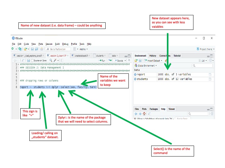
To keep or drop columns (i.e. variables) in our dataset, we use the
select() function from the dplyr package. The dplyr package will be
installed when you install the “tidyverse” – a combination of packages
we will use a lot. Make sure to always load the tidyverse for each new
session you start.
Adding dplyr:: before the select() function tells R that we want
to use the select() function from that particular package. This is
usually not needed, but there are a few functions that have the same
name but come from different packages and do different things. To go
back to our “pen” metaphor. Imagine you buy ink for your pen, you buy
two separate kinds, but coincidentally they have the same name. When you
use them, however, you realize they are in two different colors.
Before we start creating new datasets and manipulating our data, we first need to again load the required packages and import the data. We learned to do that last week.
## install if needed with install.packages("tidyverse") and load packages
library("tidyverse")

# import data

students <- readxl::read_excel("data/students.xlsx")

### dropping columns, only keeping some

report <- students %>% dplyr::select(sex, faculty, term)
Now, if you click on the new data frame that appeared on the right-hand panel, you will see that there are only 3 columns left.
Tip: report is now a new data frame. However, R can save a vast
range of different things. This is not limited to data frames. A single
number of text value can be stored (scalar) or a vector (list of data of
one data type), or a list of vectors with different data types, matrices
etc. This will be very useful later when the analysis gets more complex.
Here, I am just flagging it, if you are already curious. Find more info
on types of objects
here.
Now, let’s get rid of all students who have been at the university for
over 6 terms or do not study political science or sociology. We can do
this using the function filter() which is also part of the
tidyverse.
Note that we are using the same name for the data frame as before (i.e. “report”). This means that R will overwrite the old data frame with the same name.
We also see a couple of new elements here. First, we use %in% and we
use quotation marks in the brackets. The %in% operator tells R to
restrict the object faculty to the vector of characters defined in
c(). We define “Political Science” and “Sociology.” The whole line
would read: “Only keep students in a term that is smaller or equal to 6
AND in a faculty that is either”Political Science" or “Sociology.”
Which faculties were there again? Well, use the table() function to
find out (see last week).
Be careful! Characters (text) are case-sensitive in R. You need to always make sure your spelling is exactly how it is on your data frame. Character values (i.e. cells in columns that contain text) always need to be referenced using quotations. You do not need quotation marks for numbers.
# drop rows (i.e. observations or "cases")

report <- report %>% dplyr::filter(term<=6, faculty %in% c("Political Science", "Sociology"))
Check the report data frame again, you will see it has a lot less
“obs.” (for observations). We are basically done here. This is the list
the president wanted. But because we are nice, we will also deliver a
table summarizing the data frame.
Let’s get the sex distribution for students in both faculties (for
students for 6 or less terms). Again, there are many ways to do this,
but let’s use the tabyl function from the janitor package.
# now get the sex distribution by faculty

library(janitor) # make sure it is installed before

report %>% tabyl(faculty, sex) %>% adorn_percentages("row") %>%

  adorn_pct_formatting(digits = 1) %>%

  adorn_ns()
## faculty Female Male
## Political Science 62.3% (129) 37.7% (78)
## Sociology 51.2% (63) 48.8% (60)3.4 Sorting Rows, Ordering Columns
As we look at the data frame by clicking on the object report or by
calling str() or glimpse(), we realize that we want to arrange
the rows in an ascending order (lower terms first). We want to see
students first who have been at the university the least amount of time.
We can do this using arrange(). You can also change the order of
appearance. Call help(arrange) to see how.
# sort rows

report <- report %>% arrange(term)
Now (for whatever reason), we want the information on the faculty first,
meaning as the first column. There are different ways to change the
order of columns in R (as there are many things to do anything in R) but
one easy way is to use the select() function that you now already
know. The order in which you enter variables in the brackets is the
order in which variables will appear.
You may not care so much about the order now as the data frame is small. In future projects, you may encounter data sources with many variables where keeping similar variables next to each other or moving newly created variables up accordingly can help you in your workflow.
# change order of columns

report <- report %>% select(faculty, sex, term)
Imagine you have lots of variables, but you only want to pull some
specific variables to the front without having to type all variables
into the select() function. You can use the everything()
function. The below would read as: “Put faculty first, then sex, and
then everything else.”
# pull just one or two variables to the front

students <- students %>% select(faculty, sex, everything())
If you want to kick out only specific variables and keep the rest, you
can use the minus sign. Let’s say you do not need the variable
workingclass:
# kick out only specific variables

students <- students %>% select(everything(), -workingclass)
3.5 Changing Data Types
So far, everything went smooth. This is because all variables were already in the right format. When R isn’t happy with what you did, it will give you an error message in the console window. This happens quite a bit and, in many cases, (at least in my experience) it has to do with the type of data or variable.
Let’s try. Let’s say we want to look at life satisfaction of students.
Life satisfaction is measured from 0-100. We want to know the average
life satisfaction among all students. The command is mean():
# get the mean life satisfaction

students %>% mean(lifesat)
## Warning in mean.default(., lifesat): argument is not numeric or logical:
## returning NA## [1] NATip: If you do not use the assignment operator, it won’t save your change in the data frame. It will just produce what you asked for, in this case the mean, and display it in the console. This is a good way to simply look at stats when you do not necessarily need them later.
R gives you an error message. Why? Let’s take another look at our data
to figure out what’s wrong using glimpse(). We see that lifesat
is a “chr” variable, i.e. a character (text) variable. You cannot take
the mean of a list of character strings, you need numbers to build the
mean. So we need to convert the type of the variable. Here is one way to
do this using the mutate() function in combination with the
as.numeric() function.
# convert life satisfaction from character to numeric

students <- students %>% mutate(lifesat = as.numeric(lifesat))

glimpse(students)
## Rows: 1,000
## Columns: 22
## $ faculty <chr> "Business", "Business", "Business", "Business", "Business…
## $ sex <chr> "Male", "Female", "Female", "Male", "Male", "Male", "Fema…
## $ course <chr> "accounting", "accounting", "accounting", "accounting", "…
## $ age <dbl> 26.30697, 28.77746, 23.86429, 27.43746, 29.29478, 31.3362…
## $ cob <chr> "Spain", "Netherlands", "Netherlands", "Spain", "Germany"…
## $ gpa_2010 <chr> "3.1", "2.7", "1.7", "1.2", "3", "2.4", "3.9", "2", "0.4"…
## $ gpa_2011 <chr> "2.8", "1.2", "2.5", "2.1", "2.3", "1", "2", "0.5", "2", …
## $ gpa_2012 <chr> "2.8", "3.8", "3.8", "1.9", "1.6", "1.7", "2.3", "2.3", "…
## $ gpa_2013 <chr> "2.3", "1.8", "2.9", "1.9", "2.6", "2.4", "2.5", "1.4", "…
## $ gpa_2014 <chr> "0.5", "3", "2.4", "2.3", "3.5", "1.8", "3.4", "3.1", "4.…
## $ gpa_2015 <chr> "3.9", "3", "2.4", "4.1", "5.2", "2.6", "2.7", "3.8", "2.…
## $ gpa_2016 <chr> "3", "1.8", "1.6", "1", "1.7", "1.4", "0.1", "2.2", "1.9"…
## $ gpa_2017 <chr> "1.1", "1", "3.7", "0.8", "0.1", "1.6", "0.9", "1.3", "1.…
## $ gpa_2018 <chr> "2.6", "4", "2.8", "2.6", "2.3", "4.5", "2.3", "4.7", "3.…
## $ gpa_2019 <chr> "3.1", "2.5", "4.1", "3.4", "3.6", "3.6", "2.8", "3", "1.…
## $ gpa_2020 <chr> "3.9", "3", "5.7", "3.4", "6", "4.4", "5.7", "3.9", "4", …
## $ job <chr> "no", "no", "no", "yes", "yes", "no", "no", "no", "yes", …
## $ lifesat <dbl> 68.47224, 60.73865, 67.29213, 73.13919, 72.39454, 70.4352…
## $ like <chr> "3", "3", "4", "4", "3", "3", "2", "3", "5", "5", "5", "3…
## $ relationship <chr> "In a relationship", "Single", "In a relationship", "Sing…
## $ term <chr> "7", "4", "5", "10", "14", "13", "9", "0", "12", "3", "9"…
## $ university <chr> "Berlin", "Berlin", "Berlin", "Berlin", "Berlin", "Berlin…Life satisfaction is now “dbl” for “double.” There are two kinds of numeric data types in R: integer and double. This refers to how the data is stored and how many bits are required to store it. We don’t have to worry about that for now. For you, “dbl” or “double” simply means that we dealing with a numeric variable.
Tip: To convert variables into a character variable use
as.character() or into a factor, use as.factor().
In the command line above, we have a new, very important and powerful
element: the mutate() function. As the name gives away, it mutates
or changes things, anything really. The example above can be read as:
"Create a variable called lifesat that is equal to the numeric
version of lifesat. Since lifesat already exists, lifesat
just gets replaced with the new info.
3.6 Changing Variables
We can use mutate() to change the type of format of a variable (see
above), but mutate() is much more powerful than that. mutate()
can replace values in existing variables, rename variables, but
most importantly, it can create new variables (based on existing
ones).
3.6.1 Renaming a Variable
One way to rename a variable is simply to create a new variable which is the same than the old one, except for the name. You can leave the old variable and not be bothered by it or delete it later. For example, rename the variable “cob” to “country”:
# Rename variable "cob" into "country"

students <- students %>% mutate(country = cob)
But the best way to rename a variable is to use the rename() function. In any case, try to remember the order: new_name = old_name.
# Rename variable "cob" into "country"

students <- students %>% rename(country = cob)
3.6.2 Change/Recode Values (Cells)
What if we want to change individual values within one column/ variable?
Let’s say we want to change “UK” to “United Kingdom” in the country
variable which indicates where students are from. Note here that we are
introducing the case_when() function. This one is important and I
use it A LOT when recoding variables. In other stats languages (like
Stata) this is usually done with “if statements.”
When I read out the command line below, it would read along the lines of:
Create object students; put in it the existing object students.
Thereafter, create a column called country which is equal to “United
Kingdom” if the column cob has the value “UK.” If this
condition is not met (i.e. the cob row has other values), then the
new column country takes the same values as the existing column
country (this is what the TRUE ~ does). We simply replace certain
values within the same column.
As a result, you only change certain values. To visualize what is happening, imagine you have only one column with data. You then create an empty second column right next to it. Then you fill up the empty cells in the second column conditional on values that are available in the first column.
Note that the case_when() function has a particular grammar. Type
?case_when or help(case_when) to find out more. It uses double
= signs for values and it always uses a TRUE ~ argument at the
end.
# Replace a character value and give variable new name: Change "UK" into "United Kingdom"

table(students$cob)
##
## Austria France Germany Italy Netherlands Spain
## 91 85 153 265 54 268
## UK
## 75students <- students %>%
mutate(country = case_when(
cob=="UK" ~ "United Kingdom",
TRUE ~ country))
table(students$country)##
## Austria France Germany Italy Netherlands
## 91 85 153 265 54
## Spain United Kingdom
## 268 75The example above deals with a character variable. How does this work with numeric variables? Let’s have a look at the number of terms that students have completed (`term). Let’s also check what type of variable we got here. However, Term starts with a 0. Our supervisor tells us we should change the variable to start with a 1, because the variable was recorded in a wrong way.
# check what term is

table(students$term)
##
## 0 1 10 11 12 13 14 2 3 4 5 6 7 8 9
## 69 57 64 66 69 60 62 60 67 66 70 61 71 75 74class(students$term)## [1] "character"# Change "term" values to start at 1 not 0, give it new name
students <- students %>% mutate(term1 = as.numeric(term) + 1)
summary(students$term1)## Min. 1st Qu. Median Mean 3rd Qu. Max. NA's
## 1.000 4.000 8.000 8.026 12.000 15.000 9table(students$term, students$term1)##
## 1 2 3 4 5 6 7 8 9 10 11 12 13 14 15
## 0 69 0 0 0 0 0 0 0 0 0 0 0 0 0 0
## 1 0 57 0 0 0 0 0 0 0 0 0 0 0 0 0
## 10 0 0 0 0 0 0 0 0 0 0 64 0 0 0 0
## 11 0 0 0 0 0 0 0 0 0 0 0 66 0 0 0
## 12 0 0 0 0 0 0 0 0 0 0 0 0 69 0 0
## 13 0 0 0 0 0 0 0 0 0 0 0 0 0 60 0
## 14 0 0 0 0 0 0 0 0 0 0 0 0 0 0 62
## 2 0 0 60 0 0 0 0 0 0 0 0 0 0 0 0
## 3 0 0 0 67 0 0 0 0 0 0 0 0 0 0 0
## 4 0 0 0 0 66 0 0 0 0 0 0 0 0 0 0
## 5 0 0 0 0 0 70 0 0 0 0 0 0 0 0 0
## 6 0 0 0 0 0 0 61 0 0 0 0 0 0 0 0
## 7 0 0 0 0 0 0 0 71 0 0 0 0 0 0 0
## 8 0 0 0 0 0 0 0 0 75 0 0 0 0 0 0
## 9 0 0 0 0 0 0 0 0 0 74 0 0 0 0 0As you can see in the output of the summary() command, the new
variable term1 starts with a 1, the minimum value. To check whether
your change was correct, you can compare the old and the new variable
using a simple “cross tabulation” with the table() command.
Tip: Keep original variables that you changed at some point in your data frame. Often, you don’t know yet whether you need them again later. It is also easy to quickly double-check whether your change was correct by comparing the old variable with the new one.
Here is another example for a conditional change in a variable. Let’s
take the age of students. We get the summary of age, we see that we
have students in our dataset aged from 18 years old to 35 years old. The
average age is 26.3, half of the students are 26 or younger (median).
There are a couple new things here. First: new operators. R knows a lot of them such as plus, minus, equal (=), equal or less (<=), equal or more (>=), as well as logical operations such as “&” (and) or “|” (or). Click here for more info on operators in R.
The = sign can be confusing in R. = is sometimes used as the same as the <- operator which you have seen. Using two = signs as in == tells R to “test equality.” In other words, if you want to tell R to only do something if one object is equal to something, then you would use == (as you will see shortly).
TRUE ~ NA_real_ says that if none of the above conditions hold,
just insert NA as values. There are different types of NA values:
NA_real_ for numeric variables and NA_character for character
variables.
# let's look at the age variable

summary(students$age)
## Min. 1st Qu. Median Mean 3rd Qu. Max. NA's
## 10.00 23.67 25.85 25.92 27.98 80.00 9class(students$age)## [1] "numeric"# Creating age category variable
students <- students %>% mutate(age_category = case_when(
age >= 18 & age <=25 ~ 1,
age >25 & age<=30 ~ 2,
age >30 ~ 3,
TRUE ~ NA_real_))table(students$age_category, students$age, useNA = "ifany")Another element is the useNA element in the table() function.
Type in help(table) and you will see what this is for. Similarly, many commands have the option na.rm=TRUE or FALSE (read as “remove NA”) to specify whether to include missing observations or not.
We won’t need it now but note that you can define which values you want
to be counted as missing. Sometimes you may get survey data where the
survey company has coded values as -99 when respondents didn’t want to
answer a question. For the analysis, you can’t use that information. You
need to set it to NA, otherwise, R thinks -99 is a real number you want
to use for mathematical operations. You can conditionally assign NA
values using the function
na_if() , and
replace NA values by other values using
replace_na().
3.6.3 More Efficient Code
Above we have assigned one command line to each function in the script.
But we can be more efficient by combining these various steps into one
single command. This saves space and makes it easier to make changes
later. In the mutate() command, you can add further arguments via a
comma.
# we can do this more efficiently

students <- students %>% mutate(lifesat = as.numeric(lifesat),
                                country = cob,
                                country = case_when(
                                  cob == "UK" ~ "United Kingdom",
                                  TRUE ~ country),
                                term1 = as.numeric(term) + 1,
                                age_category = case_when(
                                  age >= 18 & age <= 25 ~ 1,
                                  age > 25 & age <= 30 ~ 2,
                                  age > 30 ~ 3,
                                  TRUE ~ NA_real_))
There you go. We did everything in one go.
There are many more ways to make code more efficient. These will be covered in later sessions. Programmers, data analysts and data scientists always try to do things with as little code as possible. However, we also have to make sure the code is still comprehensible to other people, for example, collaborators or reviewers.
Tip: Make sure to always highlight all rows you want to run. When you only highlight parts of the command, R will only run those. This can create issues sometimes.
3.6.4 Checking What Went Wrong
When you start out, it is easy to get frustrated because R gives you error messages. Errors can be the result of a small mistake, like forgetting one bracket. How do you check what went wrong (this is called de-bugging)?
Here is a quick list of things to check each time you get an error message:
Did you install the correct package and load it?
Check spelling and letter case of variable names and commands
Did you close the brackets? Are there just as many open brackets as there are closing ones?
Are you sure the variables you are using in a function are correct? If you you want to calculate a mean, for example, the variable needs to be numeric and not “chr” (character, i.e. text)
Did you previously overwrite something and are now trying to access the original?
3.7 Summarizing and Aggregating Data
In section 5 we only changed values and variables in a data frame while keeping the same overall structure. We have 1000 rows in our data frame for 1000 students. Whatever we did above, for the most part, we kept 1000 rows (except when we created the new “report” data frame with only 3 variables). Sometimes, however, we may want to summarize or aggregate certain variables which will change the overall structure of a data frame, i.e. squishing it together. When this happens, we want to save this new data frame as a new object.
For example, we have information on students’ grades in our data frame,
see column gpa_2010. This is the grade point average in 2010. Let’s
take a look at it.
# let's look at students grade point average in 2010 (gpa)

summary(students$gpa_2010)
## Length Class Mode
## 1000 character character#hhmm...doesn't work.
#let's check what type of variable it is
str(students)## tibble [1,000 × 25] (S3: tbl_df/tbl/data.frame)
## $ faculty : chr [1:1000] "Business" "Business" "Business" "Business" ...
## $ sex : chr [1:1000] "Male" "Female" "Female" "Male" ...
## $ course : chr [1:1000] "accounting" "accounting" "accounting" "accounting" ...
## $ age : num [1:1000] 26.3 28.8 23.9 27.4 29.3 ...
## $ cob : chr [1:1000] "Spain" "Netherlands" "Netherlands" "Spain" ...
## $ gpa_2010 : chr [1:1000] "3.1" "2.7" "1.7" "1.2" ...
## $ gpa_2011 : chr [1:1000] "2.8" "1.2" "2.5" "2.1" ...
## $ gpa_2012 : chr [1:1000] "2.8" "3.8" "3.8" "1.9" ...
## $ gpa_2013 : chr [1:1000] "2.3" "1.8" "2.9" "1.9" ...
## $ gpa_2014 : chr [1:1000] "0.5" "3" "2.4" "2.3" ...
## $ gpa_2015 : chr [1:1000] "3.9" "3" "2.4" "4.1" ...
## $ gpa_2016 : chr [1:1000] "3" "1.8" "1.6" "1" ...
## $ gpa_2017 : chr [1:1000] "1.1" "1" "3.7" "0.8" ...
## $ gpa_2018 : chr [1:1000] "2.6" "4" "2.8" "2.6" ...
## $ gpa_2019 : chr [1:1000] "3.1" "2.5" "4.1" "3.4" ...
## $ gpa_2020 : chr [1:1000] "3.9" "3" "5.7" "3.4" ...
## $ job : chr [1:1000] "no" "no" "no" "yes" ...
## $ lifesat : num [1:1000] 68.5 60.7 67.3 73.1 72.4 ...
## $ like : chr [1:1000] "3" "3" "4" "4" ...
## $ relationship: chr [1:1000] "In a relationship" "Single" "In a relationship" "Single" ...
## $ term : chr [1:1000] "7" "4" "5" "10" ...
## $ university : chr [1:1000] "Berlin" "Berlin" "Berlin" "Berlin" ...
## $ country : chr [1:1000] "Spain" "Netherlands" "Netherlands" "Spain" ...
## $ term1 : num [1:1000] 8 5 6 11 15 14 10 1 13 4 ...
## $ age_category: num [1:1000] 2 2 1 2 2 3 2 1 2 1 ...# ok - it is a character. We need to convert it. We know how to do that.
students <- students %>% mutate(gpa_2010 = as.numeric(gpa_2010))
str(students)## tibble [1,000 × 25] (S3: tbl_df/tbl/data.frame)
## $ faculty : chr [1:1000] "Business" "Business" "Business" "Business" ...
## $ sex : chr [1:1000] "Male" "Female" "Female" "Male" ...
## $ course : chr [1:1000] "accounting" "accounting" "accounting" "accounting" ...
## $ age : num [1:1000] 26.3 28.8 23.9 27.4 29.3 ...
## $ cob : chr [1:1000] "Spain" "Netherlands" "Netherlands" "Spain" ...
## $ gpa_2010 : num [1:1000] 3.1 2.7 1.7 1.2 3 2.4 3.9 2 0.4 4.3 ...
## $ gpa_2011 : chr [1:1000] "2.8" "1.2" "2.5" "2.1" ...
## $ gpa_2012 : chr [1:1000] "2.8" "3.8" "3.8" "1.9" ...
## $ gpa_2013 : chr [1:1000] "2.3" "1.8" "2.9" "1.9" ...
## $ gpa_2014 : chr [1:1000] "0.5" "3" "2.4" "2.3" ...
## $ gpa_2015 : chr [1:1000] "3.9" "3" "2.4" "4.1" ...
## $ gpa_2016 : chr [1:1000] "3" "1.8" "1.6" "1" ...
## $ gpa_2017 : chr [1:1000] "1.1" "1" "3.7" "0.8" ...
## $ gpa_2018 : chr [1:1000] "2.6" "4" "2.8" "2.6" ...
## $ gpa_2019 : chr [1:1000] "3.1" "2.5" "4.1" "3.4" ...
## $ gpa_2020 : chr [1:1000] "3.9" "3" "5.7" "3.4" ...
## $ job : chr [1:1000] "no" "no" "no" "yes" ...
## $ lifesat : num [1:1000] 68.5 60.7 67.3 73.1 72.4 ...
## $ like : chr [1:1000] "3" "3" "4" "4" ...
## $ relationship: chr [1:1000] "In a relationship" "Single" "In a relationship" "Single" ...
## $ term : chr [1:1000] "7" "4" "5" "10" ...
## $ university : chr [1:1000] "Berlin" "Berlin" "Berlin" "Berlin" ...
## $ country : chr [1:1000] "Spain" "Netherlands" "Netherlands" "Spain" ...
## $ term1 : num [1:1000] 8 5 6 11 15 14 10 1 13 4 ...
## $ age_category: num [1:1000] 2 2 1 2 2 3 2 1 2 1 ...summary(students$gpa_2010)## Min. 1st Qu. Median Mean 3rd Qu. Max. NA's
## 0.000 1.300 1.900 1.964 2.600 4.900 9Now, we want to create a new dataset where our rows are the courses
which students take. We want a dataset by course, and we want to know
the grade point average per course to compare the performance. To get
the average for all students, we can use the mean() function.
However, we want to get the mean by course. We first need to group the
data using group_by(). This is a VERY useful command that we will
use a lot going forward.
# This gives you the mean for all observations

mean(students$gpa_2010, na.rm = TRUE)
## [1] 1.963875# this does the same thing in a "tidyverse" framework which we have been using
students %>% summarise(mean = mean(gpa_2010, na.rm = TRUE))## # A tibble: 1 × 1
## mean
## <dbl>
## 1 1.96# now, let's group this by "course" and get the mean by course
students %>% group_by(course) %>%
summarise(mean = mean(gpa_2010, na.rm = TRUE))## # A tibble: 23 × 2
## course mean
## <chr> <dbl>
## 1 accounting 2.13
## 2 central banks 1.80
## 3 discourse 1.89
## 4 education 1.77
## 5 election 2.05
## 6 employment 1.93
## 7 EU 1.87
## 8 inequality 2.06
## 9 institutions 1.89
## 10 int. organizations 2.06
## # … with 13 more rows# let's sort it
students %>% group_by(course) %>%
summarise(mean = mean(gpa_2010, na.rm = TRUE)) %>%
arrange(mean)## # A tibble: 23 × 2
## course mean
## <chr> <dbl>
## 1 <NA> 1.56
## 2 macro I 1.62
## 3 education 1.77
## 4 leadership 1.78
## 5 central banks 1.80
## 6 marketing 1.85
## 7 EU 1.87
## 8 micro I 1.89
## 9 discourse 1.89
## 10 institutions 1.89
## # … with 13 more rowsThis looks good but we actually want this in a new data frame for later use:
course_grade <- students %>% group_by(course) %>%

  summarise(mean = mean(gpa_2010, na.rm = TRUE)) %>%

  arrange(mean)
Click on the new object course_grade. The grades for all courses
from all disciplines are not sorted. We want this by faculty AND course.
No problem, just add another level to the group_by() function:
course_grade <- students %>% group_by(faculty, course) %>%

  summarise(mean = mean(gpa_2010, na.rm = TRUE)) %>%

  arrange(mean)
In addition to the mean grade by course, we also want to know the number
of students in each course. This can be done by counting the number of
rows (each row is one student) by course. R has a convenient function
called n() for this:
# add number of observations by course

course_grade <- students %>% group_by(faculty, course) %>%

  summarise(mean = mean(gpa_2010, na.rm = TRUE),

  obs = n()) %>%

  arrange(mean)
Now we have an additional column with the number of observations per course.
Tip: The summarise() function lets you do a lot more things such as
calculating medians, minimum, maximum, quantiles and much more. Have a
look here.
Now, the dean of the university wants to compare the average grades per course with the average in the corresponding faculty and the whole department to see whether there are some courses that really stick out for being too hard or too easy. To do this, we need the average grade overall, the average by faculty and the average by course all in one dataset.
We have to use a combination of things we learned in this session to do this.
### compare grades by course, by faculty and overall

# let's keep only relevant columns

compare_grades <- students %>% dplyr::select(faculty, course, gpa_2010)

# let's create a new variable containing the mean grade in 2010 for all students

compare_grades <- compare_grades %>%

  mutate(overall_mean = mean(gpa_2010,na.rm = TRUE))

# let's create a new variable with the average by faculty

compare_grades <- compare_grades %>% group_by(faculty) %>%

  mutate(faculty_mean = mean(gpa_2010,na.rm = TRUE))

# let's create a new variable with the average by course

compare_grades <- compare_grades %>% group_by(course) %>%

  mutate(course_mean = mean(gpa_2010,na.rm = TRUE))

# now let's summarize the dataset

compare_grades <- compare_grades %>% group_by(faculty, course) %>%

  summarize(obs = n(),

  faculty_mean= mean(faculty_mean),

  course_mean= mean(course_mean),

  overall_mean = mean(overall_mean))
We are dealing with so-called nested or grouped data here. We have
students in courses and courses in faculties. When we calculate the mean
grade for all students, the new variable containing that value is the
same for all students (since there is only one mean). The same applies
to the courses. When we calculate the mean grade per course, all
students in that course have the same value in that new column. When we
created all the new means in separate variables, we then need to
condense the dataset using summarise(). This effectively means that
for some of the columns containing a constant (the same) mean in many
rows, we take the mean of a mean.
Note that taking the mean (i.e. the average) based on rows that contain the same value is (obviously) the same value. There are other ways to do this, but this one works.
Now, let us reduce this to more efficient and shorter code. Note here,
we introduced the ungroup() command which returns the data to its
previous grouping.
# condense code:

compare_grades <- students %>% dplyr::select(faculty, course, gpa_2010) %>%
  mutate(overall_mean = mean(gpa_2010,na.rm = TRUE)) %>%
  group_by(faculty) %>%
  mutate(faculty_mean = mean(gpa_2010,na.rm = TRUE)) %>%
  ungroup() %>%
  group_by(course) %>%
  mutate(course_mean = mean(gpa_2010,na.rm = TRUE)) %>%
  ungroup() %>%
  group_by(faculty, course) %>%
  summarise(
    obs = n(),
    faculty_mean= mean(faculty_mean),
    course_mean= mean(course_mean),
    overall_mean = mean(overall_mean))
3.8 Summary & keyboard shortcuts
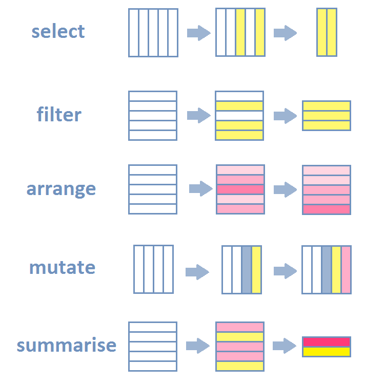
This section was quite dense. We learned the most important and most basic ways how to wrangle your data. The figure below summarizes the concepts of the main functions that I introduced in this section visually:
Before we move to the exercises, let’s look at some shortcuts that make our life
a proven 100 thousand times easier. (Source: True me.) There are ome shortcuts
you are probably already familar with, such as control/cmd (henceforth ctrl) + C
for copying, ctrl + V for pasting, and ctrl + A for selecting everything.
Now let’s move on to the R-specific shortcuts:
- on the console, you can access the last code you’ve entered by clicking on
the up arrow symbol ↑;
- ctrl + shift + M (in that order) for the pipe operater %>%;
- alt + minus sign for the assignment operator ->;
- ctrl + shift + C to comment out selected code, i.e. so that it will not be run;
- ctrl + enter will run the current line and jump to the next one, or run selected part without jumping further (You do not need to select the whole code chunk, it is sufficient to place your mouse cursor somewhere on the code line);
- ctrl + alt + R to run your whole script;
- ctrl + I to fix identation lines.
For a demonstration of some of the shortcuts mentioned here, go to this page.
3.9 Exercises I (based on class data)
Your parents call and are interested in knowing when you will finally graduate and find a job. Little do they know that you are now becoming an expert R user and can maybe use data to argue your way out of this one. In order to do so, you want to consider life satisfaction among students who work and among students who study longer than six terms.
Load the data set
studentsand create a new data frameparentswith the variables job, term and life satisfaction. Explore the data frame using theglimpse()command.You are interested in the average life satisfaction of all students regardless of their term number or job status. Luckily, we already discussed how to do this and you can review the class materials and convert the life satisfaction variable as needed. Hint: we need a numeric variable in order to calculate the mean!
Later you want to look at only Business students who are in their first year at University (There are 2 terms per year). Create a dataframe that only contains those students and their life satisfaction scores.
Now, you want to distinguish between students enrolled for longer than six terms and those enrolled for six or less. To do so, you first make sure that the term variable is numeric and starts with a 1, as we have seen in class. Then you create a new categorical variable
term_catwhich is 1 when term is equal or lower to 6 and 2 otherwise.Finally, you can compare the average life satisfaction levels of 1) all students, 2) those with and without a job, and 3) by term category. Hint: Use the
group_by()command we learned today!It looks like those students without a job and in term 7 or higher are more satisfied with their lives! What do you think?
Before you go and call back your parents, try and condense the code you wrote so far!
But then a thought suddenly occurs to you: what if students from sunny country of origins have higher life satisfaction? The additional exposure to good weather could be paramount to their happiness, and your parents must surely want you to be happy. After all, a happy students is bound to be a good student, right? Let’s figure out if your parents should send you to vacations more often!
First, we need to select the relevant variables: lifesat, term, cob. For us not to overwrite the previously created data set, we need to save it under a new object name:
parents2. Next, we need to filter out sunny countries, which also happen to be the south from Germany. Lastly, we will usesummarize()to take the mean out oflifesat.
What’s the verdict?
3.10 Exercises II (based on your own data)
Load the dataset you selected last week. Explore its variables using the
glimpse()command. Select five variables that you find interesting and create a subset and name it accordingly, for exampleweek3.Explore the five selected variable and adjust them for future use. Change at least one variable's class (meaningfully) and create one categorical variable depending on another variable's values. Hint: use the
as.numeric()andcase_whencommand!Use the
group_by()command to compare mean values between groups. Comment on your findings!
3.11 More helpful resources and online tutorials:
See Chapter 3 part 6 in this online course
See Chapter 5 in this online book
Great chapter for graduate students on data manipulation using tidyverse functions