2 Week 2: Getting started
2.1 Installing R and loading/exploring your dataset
Objective of this session:
Get you started with R
Load your first dataset in R
Explain some basic terminology and concepts
Explain how to structure any data analysis project
Learn how to run commands and save scripts
R commands covered in this session:
library()
install.packages()
read_excel()
read_xlsx()
read_csv()
commenting
head()
glimpse()
str()
summary()
table()
tabyl()
load()
save()
search()
setwd()
pipe operator (%>%)
2.2 Install R
It is likely that R is already installed on your computer if you are using one at the university. However, I still recommend installing R on your personal or work laptop for future use.
R is two things: R – the programming language (base R) – and Rstudio – the integrated development environment. Don’t worry about this now. It just means you have to install both R and Rstudio on your computer.
To install R / RStudio, watch this video or follow these steps described here. Make sure you choose the right version depending on your laptop (Windows vs. Mac; 32-bit vs. 64-bit).
2.3 First steps
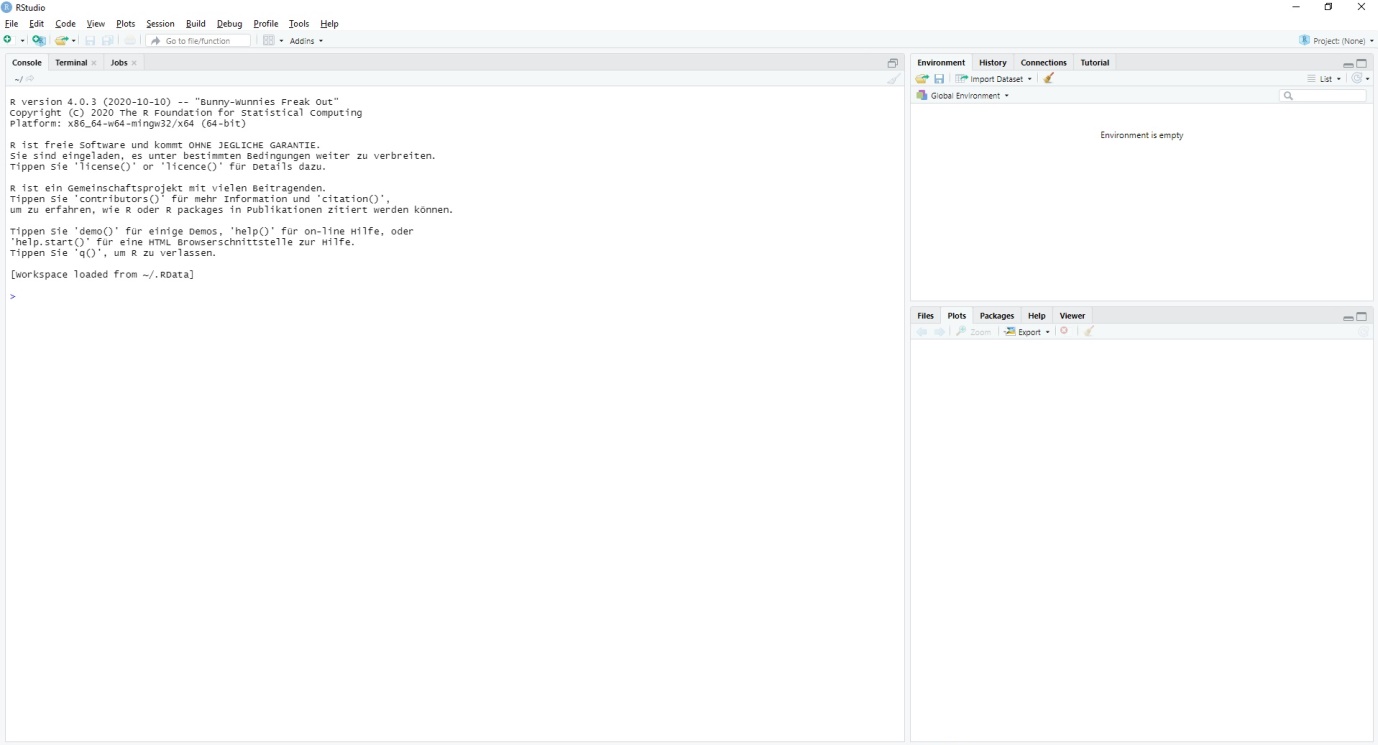
When everything is installed, run Rstudio. It should look like this:
Now, click “File,” followed by “New File” and then “R script.” The R script is your most important piece here. Rather than conducting data analysis through a “clickable” user interface (as Stata and SPSS offer), R requires “code” to run the analysis step-by-step. The R script can save your code, so do not forget to save the script as often as possible. It is basically the documentation of what you tell R to do.
Scripts have several advantages over other “clickable” interfaces: 1) They are “replicable,” i.e. others can re-do what you did. 2) If your analysis requires several steps, you don’t have to do all the steps manually over and over again. Once the script is complete, you can re-run it as many times as you like. 3) It is easier to adapt and adjust your analysis later on.
When your script is open, R should roughly look like this:
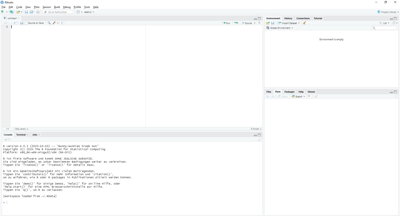
There are 4 different parts to the R user interface:
Script
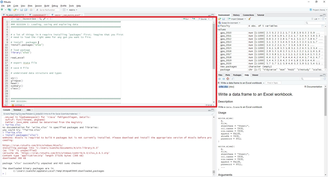
We will use the script to write code. This is the only window that we will actively change and work in. You “run” or execute a line of code with Ctrl + Enter or by using the Run button in the toolbar right above your script. This runs the currently selected line but you can run multiple lines by e.g. marking the relevant lines and running them then. Have a look here for more info on that!
Environment
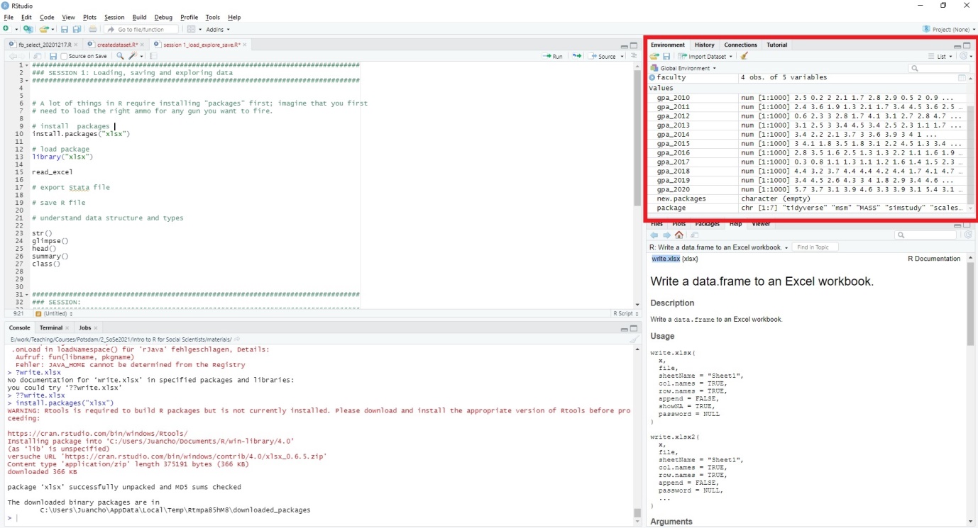
On the upper-right hand corner, you can see the “environment.” When we later save different datasets and variables, they will be listed here. Don’t worry about the content of it for now.
Plots
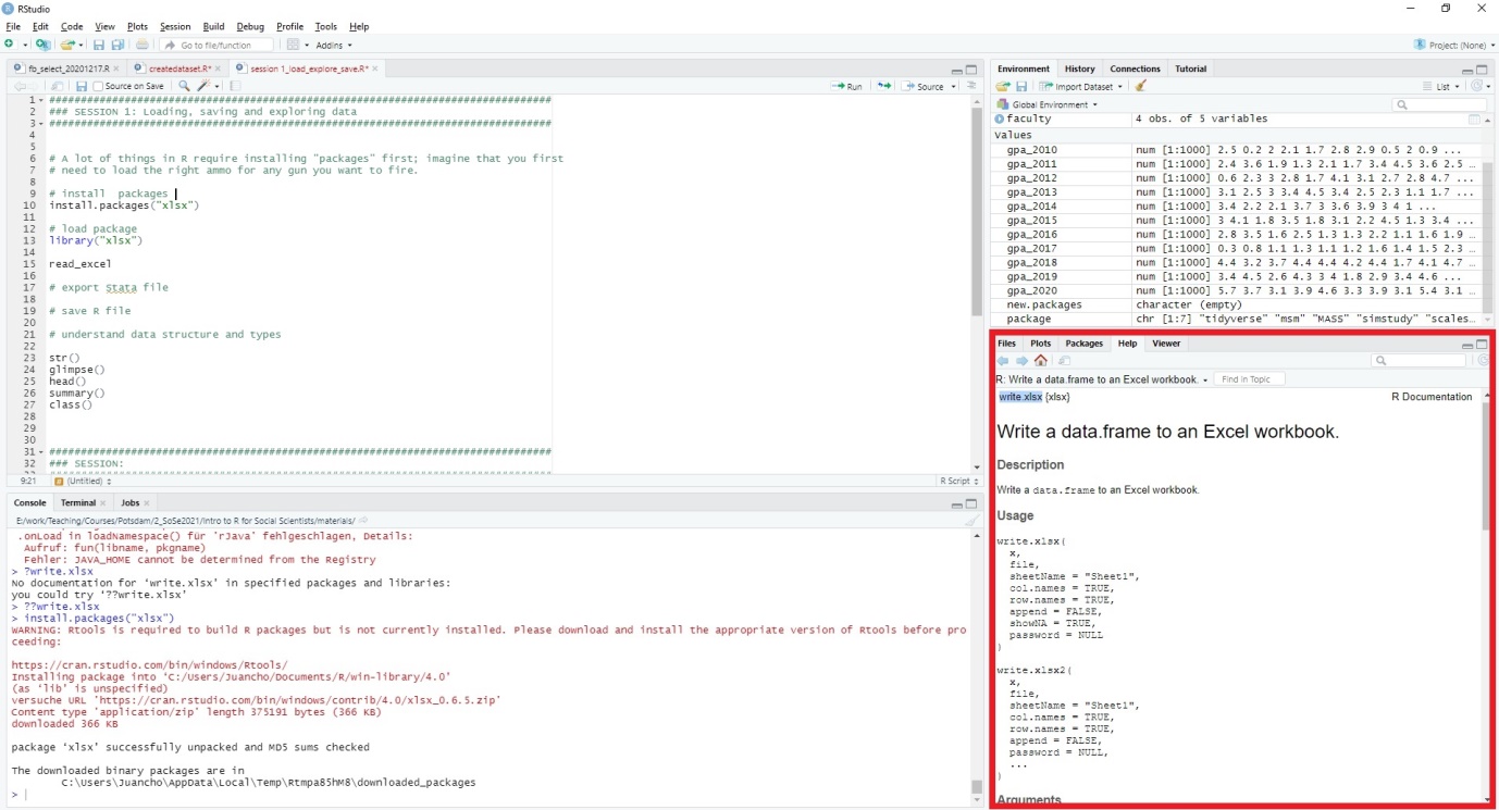
On the bottom right-hand corner, you have different sheets or tabs.
“Plots” will display any figures and plots that we produce. When you run code in the script part that produces a visual, it will be displayed here in “plots.”
Another relevant sheet/tab here is “files.” If you create an R project (more on that later), then the “files” tab will show you the files currently saved in the working folder on your computer.
You also have a “help” sheet (which is open in the visual above). You
can either search for functions/commands using the search field or run
the following things in the script or console: help(command) or
?command. The help window will open a page explaining the command or
function of interest.
Console
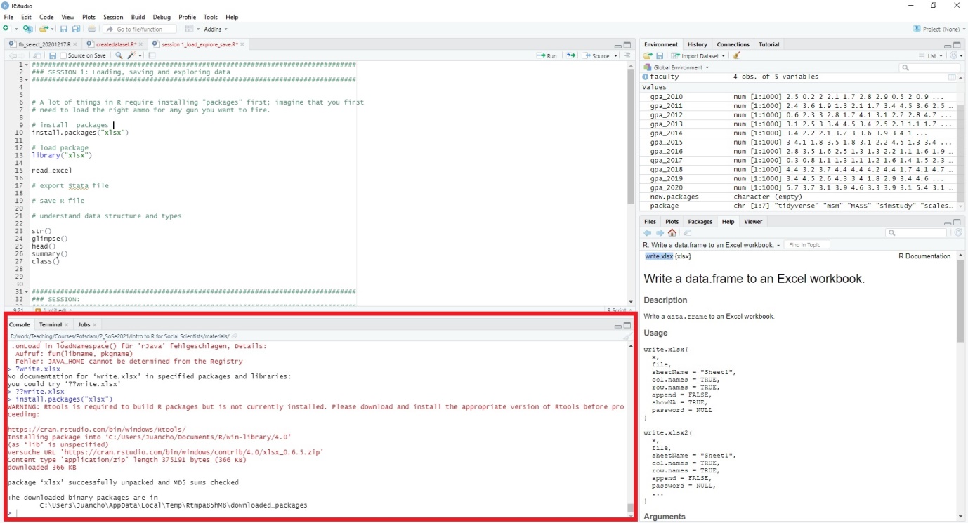
The console shows which code (that is, which lines of code) was executed. It shows you the output/ results from your analysis (except plots, they pop up in another window on the bottom right hand). This is also where warning or error messages may appear, allowing you to figure out what went wrong and/or copy paste it into Google. Don’t get intimidated by the red font, they can be quite informative! You will see very soon. Basically, don’t touch the console. You can put in commands there and run them, but there is rarely a reason to run commands only once. Stick to the script.
For review, here is a video on introducing the R interface to new users.Tip: The look of R can be adjusted in the settings, so that sometimes, the user interface might look a bit different when you watch tutorials. However, all Rstudio interfaces will have the same number and types of windows: console, plots, environment and script. Cool kids sometimes change the background color or the color of code. You can do that under Tools -> Global Settings -> Appearance.
2.4 Loading & saving
Alright, let’s get some data into R. This process is also called
“loading” data, “importing” data, “reading” data – basically they are
all the same. Before we can do that, we need to introduce two very
important commands: install.packages() and library().
Before you can do (most) things in R, you need to first install and load packages that come with a library of handy functions/operations. Imagine R is your pen. Packages are your ink. You first need to get your ink (i.e. install the package) and then put the ink in the pen (load the package) before you can start writing (execute a command). Base R (raw R without the packages) might provide you with some standard ink but other packages can provide more valuable and interesting ink. We are going to apply this to our first problem: How do we get data into R?
For that objective, we will require our first package: readxl. This package has been developed and graciously shared by Hadley Wickham and Jennifer Bryan. They have used base R to build functions that make it very easy for us to import Excel data into R.
The dataset that we will be using in this class is data on university students, so basically you. Hopefully, this will make things easier to relate to. The data is made up, so no data privacy concerns here. We are providing the data in the form of an Excel file (.xlsx) here.
Most datasets are generally available in some kind of Excel format, often it is .csv, .xls, .xlsx etc. Sometimes you may have data from other programs (stata = .dta; or SPSS).
To load an xlsx file, we need the readxl-package.
Type install.packages("tidyverse") or install.packages("readxl").tidyverseis a collection of very useful packages. When you install it,readxl` will also be installed. However, you could also just install readxl individually.
To execute a command you can press “ctrl + enter” or click on the “run” button on the top center.
Then type
# load package
library(tidyverse)
Tip: You can use the “#” sign to write a comment in the script. It is good habit to note down the steps and your thought process, because it will make it much easier to remember what intended by each step. Feel free to comment excessively like you are writing a (data) journal.
Now, the command is ready to be executed:
students <- readxl::read_excel("data/students.xlsx")To import a .csv file, you do not need to install a certain package. It already comes with the default library in your Rstudio:
students <- read.csv("data/students.csv")When you import data into R, you need to give the dataset a name. That
name is the label of the object. Anything can be an object. An object is
basically a container where something is stored. Could be data, a list
of things, a number or variables. Here, we have created a the object
with the label “students.” <- is the assignment operator, by
which we are assigning the dataset to the variable “students.” R then
knows that every time you use the name you reference the previously
loaded dataset. This calls for caution: unless you want to overwrite it,
do not use the same name twice! You also need to tell the function where
the Excel file is located. In my case, the file is saved in the directory “data.” You would need to change this and include the path to the folder where you saved the file.
There is a more convenient way to specify the location of files on your computer
using setwd() (i.e. "set working directory). You define it once and then R
knows where your files are. Then, you only need to put the name of the files in the relevant command.
setwd("your path here")
students <- readxl::read_excel("yourfilename.xlsx")
In our command line (code), we are telling R to read the excel file and then store it in the object “students.” R usually automatically recognizes what you want to store in an object. In this case, we want to store a dataset. R calls datasets data frames.
You have successfully loaded a data frame into R. Imagine you’ve done some manipulations to the data frame. It is time to save your new output as “.RData” as follows:
save(students, file = "path/to/folder/students.RData")Here, you first say which loaded file you would like to save and then specify the file name in “….” You can load an “.RData” file using load(). Note here, that you do not need to specify a name here: load("data/students.RData") will load the “students.RData” file from the “data” folder and add it to your environment under its given name “students” automatically.
Alternatively, you can also save it as a “.xlsx” or “.csv” file:
install.packages("openxlsx")
write.xlsx(students, file = "path/to/folder/students.xlsx")
# no need for a package here as this function it in-built, i.e. already included
write.csv(students,"path/to/folder/students.csv")Important: For some sadistic reason, R only accept forward slashes (“/”), not backward slashes (“\”). When you copy a location from your folder directory, the slashes are often backward. So make sure you change them. Otherwise, R won’t read the location correctly and cannot find your data.
Tip: type in library() to see all packages that are currently
installed. Type in search() to see packages currently loaded. You
only have to install packages once, but you need to load them once in
every new session.
Additional resources on importing data:
For information on importing Stata, SPSS or csv file, please click here.
2.5 Explore your dataset
The most important step before running any analysis or producing fancy visuals is to understand what kind of data you are dealing with. R will help you run the analysis and make your graphs look pretty, but it cannot help you decide what you should and should not be doing with your data. Exploring your data is a key first step.TIPP: In the meanwhile, save your script again! Look for “Save as” in the “File” header, give it a name and save it your working folder. Make sure you regularly save your script. A useful shortcut is “ctrl + s.” You absolutely do not want to start from the beginning in case your computer crashes or freezes. Trust me.
So, let’s see what we are dealing with:
Head() gives you a sneak preview of what the first 6 rows of your
dataset looks like. str() gives you the “structure” of the dataset.
A “tibble” is another name for “tidy dataset,” meaning that the data is
organized in structured, clear rows and columns. “(1,000 x 12)” means
that the dataset contains 1000 rows and 12 columns. Commonly, in social
sciences, rows are referred to as “observations” and columns as
“variables.” In our case, there are 1000 observation to each of the
12 variables.
# look at the first 6 rows of the dataframe
head(students)
## # A tibble: 6 × 23
## faculty course age cob gpa_2010 gpa_2011 gpa_2012 gpa_2013 gpa_2014
## <chr> <chr> <dbl> <chr> <chr> <chr> <chr> <chr> <chr>
## 1 Business accounti… 26.3 Spain 3.1 2.8 2.8 2.3 0.5
## 2 Business accounti… 28.8 Netherl… 2.7 1.2 3.8 1.8 3
## 3 Business accounti… 23.9 Netherl… 1.7 2.5 3.8 2.9 2.4
## 4 Business accounti… 27.4 Spain 1.2 2.1 1.9 1.9 2.3
## 5 Business accounti… 29.3 Germany 3 2.3 1.6 2.6 3.5
## 6 Business accounti… 31.3 Italy 2.4 1 1.7 2.4 1.8
## # … with 14 more variables: gpa_2015 <chr>, gpa_2016 <chr>, gpa_2017 <chr>,
## # gpa_2018 <chr>, gpa_2019 <chr>, gpa_2020 <chr>, job <chr>, lifesat <chr>,
## # like <chr>, relationship <chr>, sex <chr>, term <chr>, university <chr>,
## # workingclass <chr># explore structure dataset
str(students)## tibble [1,000 × 23] (S3: tbl_df/tbl/data.frame)
## $ faculty : chr [1:1000] "Business" "Business" "Business" "Business" ...
## $ course : chr [1:1000] "accounting" "accounting" "accounting" "accounting" ...
## $ age : num [1:1000] 26.3 28.8 23.9 27.4 29.3 ...
## $ cob : chr [1:1000] "Spain" "Netherlands" "Netherlands" "Spain" ...
## $ gpa_2010 : chr [1:1000] "3.1" "2.7" "1.7" "1.2" ...
## $ gpa_2011 : chr [1:1000] "2.8" "1.2" "2.5" "2.1" ...
## $ gpa_2012 : chr [1:1000] "2.8" "3.8" "3.8" "1.9" ...
## $ gpa_2013 : chr [1:1000] "2.3" "1.8" "2.9" "1.9" ...
## $ gpa_2014 : chr [1:1000] "0.5" "3" "2.4" "2.3" ...
## $ gpa_2015 : chr [1:1000] "3.9" "3" "2.4" "4.1" ...
## $ gpa_2016 : chr [1:1000] "3" "1.8" "1.6" "1" ...
## $ gpa_2017 : chr [1:1000] "1.1" "1" "3.7" "0.8" ...
## $ gpa_2018 : chr [1:1000] "2.6" "4" "2.8" "2.6" ...
## $ gpa_2019 : chr [1:1000] "3.1" "2.5" "4.1" "3.4" ...
## $ gpa_2020 : chr [1:1000] "3.9" "3" "5.7" "3.4" ...
## $ job : chr [1:1000] "no" "no" "no" "yes" ...
## $ lifesat : chr [1:1000] "68.4722360275967" "60.7386549043799" "67.2921321180378" "73.1391944810778" ...
## $ like : chr [1:1000] "3" "3" "4" "4" ...
## $ relationship: chr [1:1000] "In a relationship" "Single" "In a relationship" "Single" ...
## $ sex : chr [1:1000] "Male" "Female" "Female" "Male" ...
## $ term : chr [1:1000] "7" "4" "5" "10" ...
## $ university : chr [1:1000] "Berlin" "Berlin" "Berlin" "Berlin" ...
## $ workingclass: chr [1:1000] "yes" "yes" "no" "yes" ...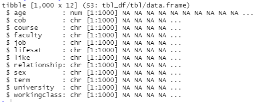
Tip: With your mouse, go to the environment panel (upper-right) and click on the “students” object. It pops up and you can browse through it. This is often a good idea to get a first feel for the data, but only recommended if your dataset is relatively small.
In the second row, we see listed underneath each other the list of
“variables” or “column” names: age, cob (short for country of birth),
course, faculty, job, lifesat (life satisfaction as in how satisfied are
students with their classes), relationship status, sex, term,
university, workingclass.
After the column name, we see the data “type” – which is of very high importance – and the first 4-5 values in the dataset.
2.5.1 Data types
Data can occur in many forms, but for this lesson, we are going to focus on two specific data types: numeric and character. Numeric variables represent numeric numbers with which you can perform mathematical operations. Character variables represent strings or sequences of characters, including letters, symbols and numbers. The data type defines the operations that are possible with the one data type, i.e. the meaning of the data. For example, we can take the mean of numeric variables, but we cannot take the mean of character variables.
Think of data types as different cutlery in your drawer. Stay with me here for a second, I won’t give up this metaphor just yet: If you want to eat a soup, you need a spoon. A fork won’t help you. If you need to cut something, you need a knife and you will have a hard time using a spoon to cut a piece of meat. It is the same with data types in your dataset. You need to understand the type of variable before you use it for something. This will prevent a lot of frustration later on because R gives you an error message every time you try to use a fork to eat a soup (i.e. you want to, for example, get the average of a character variable).
There are the following types in R:
character: "a", "swc", "6_21", "This is also a string of characters, symbols, etc.!"
numeric: 2, 15.5 (can be real or decimal)
integer: 2LB (the L tells R to store this as an integer)
logical: TRUE, FALSE
complex: 1+4i (complex numbers with real and imaginary parts)
You can also use glimpse() to get a little bit more info about the
range of values:
glimpse(students)## Rows: 1,000
## Columns: 23
## $ faculty <chr> "Business", "Business", "Business", "Business", "Business…
## $ course <chr> "accounting", "accounting", "accounting", "accounting", "…
## $ age <dbl> 26.30697, 28.77746, 23.86429, 27.43746, 29.29478, 31.3362…
## $ cob <chr> "Spain", "Netherlands", "Netherlands", "Spain", "Germany"…
## $ gpa_2010 <chr> "3.1", "2.7", "1.7", "1.2", "3", "2.4", "3.9", "2", "0.4"…
## $ gpa_2011 <chr> "2.8", "1.2", "2.5", "2.1", "2.3", "1", "2", "0.5", "2", …
## $ gpa_2012 <chr> "2.8", "3.8", "3.8", "1.9", "1.6", "1.7", "2.3", "2.3", "…
## $ gpa_2013 <chr> "2.3", "1.8", "2.9", "1.9", "2.6", "2.4", "2.5", "1.4", "…
## $ gpa_2014 <chr> "0.5", "3", "2.4", "2.3", "3.5", "1.8", "3.4", "3.1", "4.…
## $ gpa_2015 <chr> "3.9", "3", "2.4", "4.1", "5.2", "2.6", "2.7", "3.8", "2.…
## $ gpa_2016 <chr> "3", "1.8", "1.6", "1", "1.7", "1.4", "0.1", "2.2", "1.9"…
## $ gpa_2017 <chr> "1.1", "1", "3.7", "0.8", "0.1", "1.6", "0.9", "1.3", "1.…
## $ gpa_2018 <chr> "2.6", "4", "2.8", "2.6", "2.3", "4.5", "2.3", "4.7", "3.…
## $ gpa_2019 <chr> "3.1", "2.5", "4.1", "3.4", "3.6", "3.6", "2.8", "3", "1.…
## $ gpa_2020 <chr> "3.9", "3", "5.7", "3.4", "6", "4.4", "5.7", "3.9", "4", …
## $ job <chr> "no", "no", "no", "yes", "yes", "no", "no", "no", "yes", …
## $ lifesat <chr> "68.4722360275967", "60.7386549043799", "67.2921321180378…
## $ like <chr> "3", "3", "4", "4", "3", "3", "2", "3", "5", "5", "5", "3…
## $ relationship <chr> "In a relationship", "Single", "In a relationship", "Sing…
## $ sex <chr> "Male", "Female", "Female", "Male", "Male", "Male", "Fema…
## $ term <chr> "7", "4", "5", "10", "14", "13", "9", "0", "12", "3", "9"…
## $ university <chr> "Berlin", "Berlin", "Berlin", "Berlin", "Berlin", "Berlin…
## $ workingclass <chr> "yes", "yes", "no", "yes", "yes", "no", "no", "no", "yes"…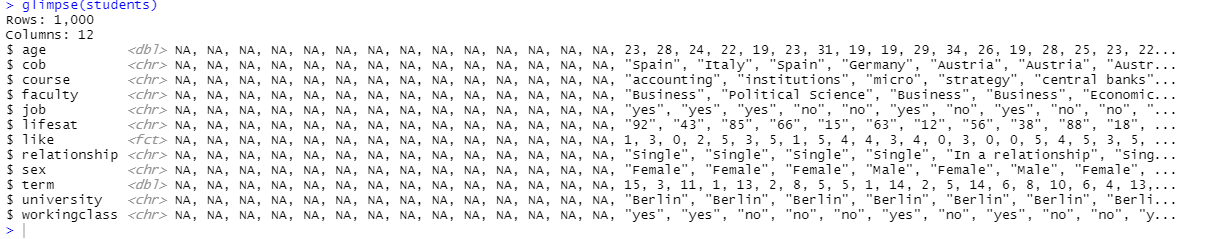
In addition, to the first rows, you now also have the range of values included in each row on the right-hand side.
When you are not sure what an object in R is (and you don’t want to see
the whole dataset using str(), type class(). For example, let’s
try it with our dataset “students”:
class(students)## [1] "tbl_df" "tbl" "data.frame"This tells you that the object students is of the type data frame.
Let’s try it on a column:
class(students$age)## [1] "numeric"This tells you that the object age in the dataframe students is
numeric. The $ sign extracts items from a list based on their names. In
our case, we extracted the column based on its name from the dataframe
students. R allows you to load many datasets at the same time. This
is why you always need to specify which dataset you are referring to.
class(students$cob)## [1] "character"Now we tried it with cob. The object is of the character type,
meaning it entails letters and probably refers to the country of birth
for every student in our data.
The summary() command will get you a “summary” of the whole dataset:
summary(students)## faculty course age cob
## Length:1000 Length:1000 Min. :10.00 Length:1000
## Class :character Class :character 1st Qu.:23.67 Class :character
## Mode :character Mode :character Median :25.85 Mode :character
## Mean :25.92
## 3rd Qu.:27.98
## Max. :80.00
## NA's :9
## gpa_2010 gpa_2011 gpa_2012 gpa_2013
## Length:1000 Length:1000 Length:1000 Length:1000
## Class :character Class :character Class :character Class :character
## Mode :character Mode :character Mode :character Mode :character
##
##
##
##
## gpa_2014 gpa_2015 gpa_2016 gpa_2017
## Length:1000 Length:1000 Length:1000 Length:1000
## Class :character Class :character Class :character Class :character
## Mode :character Mode :character Mode :character Mode :character
##
##
##
##
## gpa_2018 gpa_2019 gpa_2020 job
## Length:1000 Length:1000 Length:1000 Length:1000
## Class :character Class :character Class :character Class :character
## Mode :character Mode :character Mode :character Mode :character
##
##
##
##
## lifesat like relationship sex
## Length:1000 Length:1000 Length:1000 Length:1000
## Class :character Class :character Class :character Class :character
## Mode :character Mode :character Mode :character Mode :character
##
##
##
##
## term university workingclass
## Length:1000 Length:1000 Length:1000
## Class :character Class :character Class :character
## Mode :character Mode :character Mode :character
##
##
##
## As we can see, this only works for numeric variables. R gives you the mean, median and so forth. It does not work on the other columns/ variables because some of them are still (erroneously) defined as character objects. Let’s change that quickly, run this (don’t worry about it for now):
students <- students %>%   mutate(like = as.factor(like),
                                  term = as.numeric(term))
Let’s try the summary command again:
summary(students)## faculty course age cob
## Length:1000 Length:1000 Min. :10.00 Length:1000
## Class :character Class :character 1st Qu.:23.67 Class :character
## Mode :character Mode :character Median :25.85 Mode :character
## Mean :25.92
## 3rd Qu.:27.98
## Max. :80.00
## NA's :9
## gpa_2010 gpa_2011 gpa_2012 gpa_2013
## Length:1000 Length:1000 Length:1000 Length:1000
## Class :character Class :character Class :character Class :character
## Mode :character Mode :character Mode :character Mode :character
##
##
##
##
## gpa_2014 gpa_2015 gpa_2016 gpa_2017
## Length:1000 Length:1000 Length:1000 Length:1000
## Class :character Class :character Class :character Class :character
## Mode :character Mode :character Mode :character Mode :character
##
##
##
##
## gpa_2018 gpa_2019 gpa_2020 job
## Length:1000 Length:1000 Length:1000 Length:1000
## Class :character Class :character Class :character Class :character
## Mode :character Mode :character Mode :character Mode :character
##
##
##
##
## lifesat like relationship sex
## Length:1000 1 : 90 Length:1000 Length:1000
## Class :character 2 :199 Class :character Class :character
## Mode :character 3 :263 Mode :character Mode :character
## 4 :248
## 5 :144
## 6 : 47
## NA's: 9
## term university workingclass
## Min. : 0.000 Length:1000 Length:1000
## 1st Qu.: 3.000 Class :character Class :character
## Median : 7.000 Mode :character Mode :character
## Mean : 7.026
## 3rd Qu.:11.000
## Max. :14.000
## NA's :9We now see that two more numerical variables are there: term and
like. Term is the number of terms that the student has been enrolled
at university. summary() will give you the mean and median in addition
many more statistics. like is the measure for how much students are
fond of their class. This variable is a factor variable. It is very
important to understand
factor
variables. Factors are used to represent categorical data.
Another distinction of data types available is the one between continuous and categorical data. Categorical variables contain a finite number of categories or distinct groups. They might or might not have a logical order. An example of an ordered categorical variable (ordinal) can be a Likert scale with five levels: “Strongly Disagree,” “Disagree,” “Neutral,” “Agree,” “Strongly Agree.” An example of an unordered categorical variable (nominal) can be ice cream types or weekdays. Continuous variables are numeric variables that have an infinite number of values between any two values. Examples of continuous variables are length, temperature, weight, and speed.
Factors are an important class for statistical analysis and for plotting. Factors can both take on the form of integers or characters. They have labels associated with these unique integers or characters.
Detour: In our example, the values 1-6 in our like variable
represent different levels of liking the class from 1 = “I hate it” to 6
“I love it” – a typical likert variable. If the cells contained “I hate it” written in characters, then it would be more obvious that we are dealing with a character
variable. Because the world isn’t fair, the character levels were
converted into numbers 1-6 before the dataset was created and shared
with us. Now, R is in a weird position. It has numerical values in the
like variable but thinks that it is text. This often happens because
when we import data from Excel files, sometimes variables do not take up
the type of variable that we think it should. We will learn later how to
convert types.
If you have a large dataset, maybe you only want to look at a few variables:
# let's do it for specifc vars
summary(students$like)
## 1 2 3 4 5 6 NA's
## 90 199 263 248 144 47 9summary(students$term)## Min. 1st Qu. Median Mean 3rd Qu. Max. NA's
## 0.000 3.000 7.000 7.026 11.000 14.000 9What if you want to look at specific non-numeric categorical variables
(i.e. string/character)? You can use table() to get a feel for
those. table() returns a one-way frequency table, i.e. the count of
observations for each category of the variable (see next section). As a refresher: It is
very important to understand the type of variable that you are dealing
with. The most important ones are:
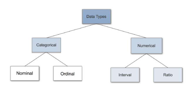
Categorical: e.g. Education, sex, religion
Nominal: e.g. religion (no clear order)
Ordinal: e.g. school grades (A, B ,C)
Numerical (continuous): e.g. age, income, satisfaction etc.
Tip: Think about questions in common surveys that you have come across in the past. Which types should they be in our data frame?
2.5.2 Data structures
The data type defines the operations that are possible with the one data type, i.e. the meaning of the data. Data structures, on the other hand, define the way data (one or multiple types) is stored and the operations that are possible with the data type(s).
Now on to data structures. For this class, you will only need to know 2:
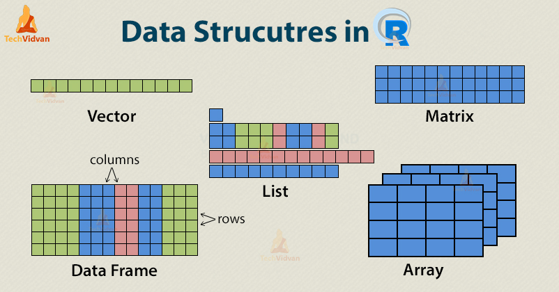
vectors and data frames. Still, this is useful to know! To reiterate, data
structures define the way data is stored and the operations that are possible
with the data type(s). Vectors combine data of one type (indicated by the colors
in the picture above) and are one/single-dimensional. You can create a vector
using the function c().
# let's create vectors
vector1 <- c(1, 2, 3)
vector2 <- c("random", "words", "here")
vector3 <- c(FALSE, TRUE, TRUE, FALSE)
vector4 <- c(1.6, 4.5, 0.55, -10)
Do you know what data types the vectors above contain?
Maybe you just want to take the average (mean) of the first and last vector. Or the first two letters of the second vector. For these relatively simple tasks, vectors are perfect.
By contrast, data frames can combine several data types and are two-dimensional: instead of only one row or column, we can now store information in both multiple
rows and columns of the same length. To create a data frame, we can use the
easy-to-remember and handy data.frame() function.
# let's create a dataframe
dataframe <- data.frame(vector1, vector2, vector3, vector4)
This will not work. We will receive an error message. Try it out yourselves: copy the code into your console and run it. A data frame requires the same number of items for each column and each row. It is not possible to introduce columns with 3 rows and 4 rows respectively into a data frame. Let’s correct that, shall we?
# let's create a dataframe
dataframe <- data.frame(vector1, vector2,
                        vector3 = c(FALSE, TRUE, TRUE),
                        vector4 = c(1.6, 0.55, -10))
Data frames are useful for storing complex information: information that is not one-dimensional. An example would be an address book, containing character data (name, address, city name, etc.), numeric data (phone number, postal code, coordinates, etc.), float data (internet IP address, etc.), logical data (wants to receive ads: FALSE/TRUE, etc.), etc.
Matrices are also two-dimensional but can only contain one data type. Finally, lists can consist of vectors of various lengths and data types.
2.5.3 Look at variables
So let’s try it.
These functions will get you the frequency table for the variable
“country of birth.” The first command includes missing information
(labelled as NA), the second one excludes missing information. Missing
values are values that ... well …. are missing. Maybe the student did
not provide that information when they enrolled, so we simply have no
information about the country of birth for some of them. To include the
missing values, add the argument useNA = "ifany" to the table()
function. There are other things you can add. Type in help(table) to
find out more.
# look at specific variables
table(students$cob)
##
## Austria France Germany Italy Netherlands Spain
## 91 85 153 265 54 268
## UK
## 75table(students$cob, useNA = "ifany")##
## Austria France Germany Italy Netherlands Spain
## 91 85 153 265 54 268
## UK <NA>
## 75 9Let’s try another package to get more info on univariate (just one
variable) and bivariate (2 variables) descriptive statistics. First, we
need to install the janitor package with install.packages("janitor"). Then let’s call the tabyl()
function. In addition to the frequency, this will return the proportion
in percent. Next to how many students were born in what country, how
many percent of students were born in each country (e.g. 25% for Italy).
In other words, the function returns the absolute and relative frequency
distribution.
# let's try another package
library("janitor")
tabyl(students$cob)
## students$cob n percent valid_percent
## Austria 91 0.091 0.09182644
## France 85 0.085 0.08577195
## Germany 153 0.153 0.15438951
## Italy 265 0.265 0.26740666
## Netherlands 54 0.054 0.05449041
## Spain 268 0.268 0.27043391
## UK 75 0.075 0.07568113
## <NA> 9 0.009 NALet’s try to look at two variables using a crosstab(ublation). A crosstab displays the relationship between two or more variables by returning the number of observations with each combination of possible values of the two variables in each cell of the table.
Here, we get to see how many men and women are in each faculty. As before, the first example includes NA values and the second one excludes NA values.
# cross-tabular (2 variables)
students %>% tabyl(sex, faculty)
## sex Business Economics Political Science Sociology NA_
## Female 131 74 161 78 3
## Male 205 149 103 80 7
## <NA> 3 2 0 4 0# do not show missings
students %>% tabyl(sex, faculty, show_na = FALSE)## sex Business Economics Political Science Sociology
## Female 131 74 161 78
## Male 205 149 103 80There is one new weird sign here: %>%. This thing is called a
“pipe” or the pipe operator. You will love it because it makes your
life easier. You can read it as telling R: “first do this and then do
that.” So, first you tell R to use the object “students” and then
(%>%) you tell R to take that object and perform the tabyl()
operation with that object. Pipes makes it easier to comprehend the
order of steps in operations and makes reading code more intuitive in
some cases.
Now, let’s add the percentages. First use the help() function to see
how to do that.
# as percentages
help(tabyl)
?tabyl

students %>% tabyl(sex, faculty, show_na = FALSE) %>%
  adorn_percentages("row") %>%
  adorn_pct_formatting(digits = 1) %>%
  adorn_ns()
## sex Business Economics Political Science Sociology
## Female 29.5% (131) 16.7% (74) 36.3% (161) 17.6% (78)
## Male 38.2% (205) 27.7% (149) 19.2% (103) 14.9% (80)See how the piping works here. You can pipe as many times as you wish. Each time something is added to the things you did before.
Adorn_pct_formatting(digits=1) tells R to report all decimal
numbers with just one digit.
Tipp: Before it is your turn to get coding, I would like to remind you of two very important tips:
Run help(command) and a window will pop up that explains how each
command works.
Even more important: Google until your fingers bleed. There are millions of R users out there. They all have started where you are now. Most questions have been answered in online fora or addressed through a tutorial. Google: “How to ….in R” or “R table” or “R import data” etc.
2.6 Data used in the course
The data used in the course consists of 4 randomly generated datasets.
The students dataset entails demographic and school-related information on imaginary students, such as
- faculty: Business, Economics, Political Science, Sociology
- course: accounting, migration, statistics. leadership, marketing, math, etc.
- age: range from 10 to 80 (There are no limits!)
- cob (country of birth): Netherlands, Germany, Uk, etc.
- gpa_2010 - gpa_2020: Grade Point Average (average mark) from 0 to 6
- job: yes for job, no for no job
- lifesat: general life satisfaction from 0 to 100
- like: perceived satisfaction with course from 1 to 6
- relationship: In a relationship or Single
- sex: Male or Female
- term: from 1 to 14
- university: Berlin
- workingclass: yes for working class background, no for no working class background
The students2 dataset deviates from the students dataset only in formatted design in Excel.
The faculty dataset contains aggregated data per faculty:
- faculty: Business, Economics, Political Science, Sociology
- students: number of students
- profs: number of profs
- salary: amount of salary
- costs: amount of costs
The course dataset depicts information on the individual courses.
- course: accounting, employment, EU, leadership, theory, etc.
- students: number of students
- profexp: years of experience by professor
- profsex: Male or Female professor
- deliverable: exam, paper or presentation
- timing (of course): 10 am, noon, 2 pm, etc.
2.7 Exercises I (based on class data)
Download R and R Studio and get a feeling for the interface. It's not that scary!
Open a new R script and load the student data as we just did in class. A new object called
studentsnow appears in the environment panel (upper right), click it if you wish to have a closer look on the data!Explore the data set by running the commands
head(students),str(students),glimpse(students)andsummary(students)in your R script. You will use these a lot in the future, so have a closer look at the different outputs in the console (lower left). Remember to save your script!Now focus on the variables
age,jobandrelationship. Find out more about their type! If the variable is numeric, have a look at its summary, if not create a table to get to know them better. Hint: be mindful about missing observations!Finally, create a cross-tabulation of the variables
jobandrelationshipusingtabyl()from the janitor package. Do not show the missing observations!Re-create the table using percentages with two digits and numbers of observations in brackets. Hint: Look at the command we used in class and add each piped line step by step to understand what each line does!
2.8 Exercises II (based on your own data)
Think about a topic or question you are interested in (Hobbies? Geek interest? Political agenda?). Then think about some data that could be relevant for the subject. See if you find data online that is publicly accessible. Download it, import it into R and explore it. Get an overview of what types of variables and observations are in there. Save your script and submit it on moodle. In the coming weeks, think hard about a dataset that could really interest you for the duration of this course. It will make it easier if you work on it alongside this course. It will keep you motivated. Each week you will get short exercises to complete using your own dataset.
If you cannot think of any data, here are some suggestions you could explore:
Free but requiring registration
Eurobaromter (public opinion survey)
World Values Survey (public opinion survey)
PEW research (politics, journalism, public opinion)
Publicly accessible
On a side note, sometimes R does not recognize a variable, for example when its name starts with a number or includes spaces. In those cases, simply use backticks around the variable (e.g. `2018 GDP`) when refering to it.